Introduction
Motivation
Indeed, much high-profile progress has leveraged these tools to learn complex behaviors from data and/or simulations [80, 151]. For example, in the Rubiks cube example mentioned above, the robotic hand managed to solve the Rubiks cube 20% of the time [9]; in the ranking example, the system managed to capture successfully 96% of the time [94].
Problem Statement
The first half of Chapter 5 examines various uncertainty models used to predict human behavior and guarantee safety in multiagent settings; it discusses how and why these models fall short in safety-critical applications due to the unique nature of human uncertainty. The second half of Chapter 5 examines how to leverage and encode prior knowledge of human behavior and intent to provide safety guarantees in multiagent, human settings based on more accurate, interpretable modeling assumptions.
Related Work
This allows us to exploit many of the benefits of model-based RL without being so sensitive to model inaccuracies. Model-based reinforcement learning: Model-based RL algorithms, on the other hand, learn a model of the environment, which they use to learn the optimal policy (or value function) [122].
Contributions and Structure of this Thesis
Recall that in the MDP model (2.1), the system dynamics were described by the mapping 𝑓(𝑎): 𝑆 × 𝐴 → 𝑆, which is unknown to the learning agent. In the driving scenario, the optimal model simplifies to the Gaussian distribution, since 𝑄𝐻 = k𝑥𝑡+1−𝑥ˆ𝑡+1kΣ for someΣ (i.e., the best fit to the data is sought).
Background and Preliminaries
Reinforcement Learning
In 1992, Williams [178] showed that the following expression represents an unbiased estimator for the policy gradient. Let us refer to the policy𝜋𝜃 as “actor” and the action value function𝑄𝜋𝜃 as.
Control Barrier Functions
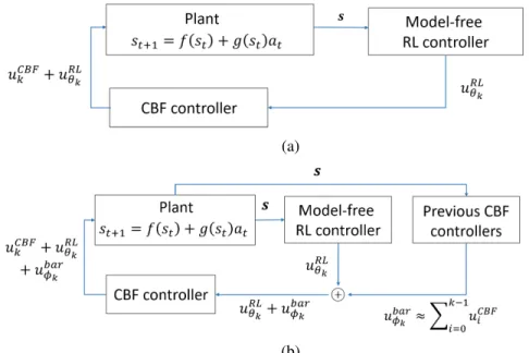
However, due to the close dependency between the actor and the critic, the update step sizes must be chosen carefully to avoid learning instability. The existence of a CBF implies that there exists adeterministic controller 𝑢𝐶 𝐵 𝐹 : 𝑆 → 𝐴 such that setCis is forward invariant with respect to the system dynamics.
Gaussian Process Models
With this model of the posterior distribution over 𝑑(𝑠), high probability confidence intervals on the function can be easily calculated. This limitation is easily overcome by using a separate GP model for each dimension of the output function, 𝑑 [173].
Mathematical Notation
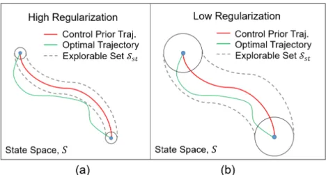
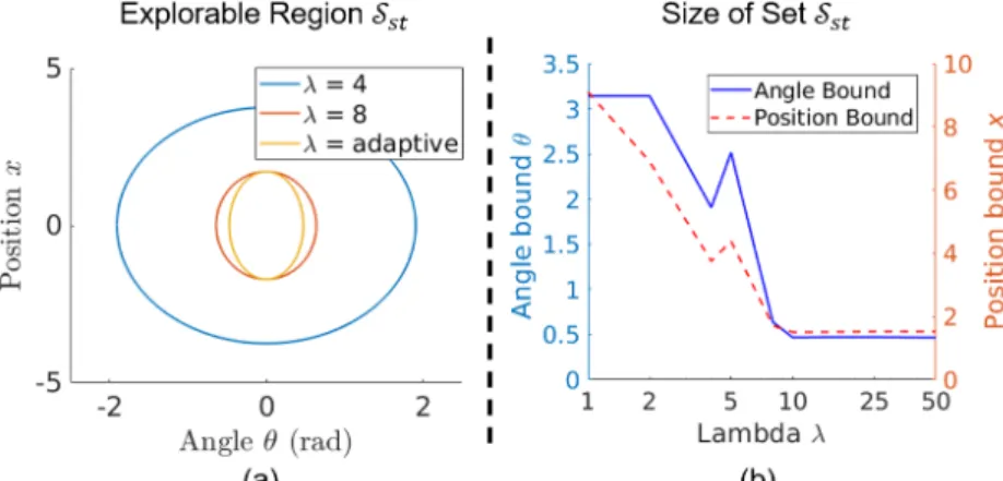
The optimal trajectory for a desired task is likely to deviate from the nominal trajectory (i.e., the control theoretical trajectory), as shown in Figure 3.2 – the setS𝑠𝑡 illustrates the explorable area under regularization. As a result, the problems illustrated in Figures 5.2 and 5.3 are exactly confronted by the noisy rational model (that is, the shape of the underlying distribution does not match the assumed distribution).
![Figure 3.1: Learning curves for 6 separate learning trials when using the RL algorithm DDPG [150] to solve the CartPole task in the OpenAI gym environment](https://thumb-ap.123doks.com/thumbv2/123dok/10402451.0/33.918.223.654.518.762/figure-learning-separate-learning-algorithm-cartpole-openai-environment.webp)
Control Regularization for Reinforcement Learning
Reducing Variance in RL through Control Regularization
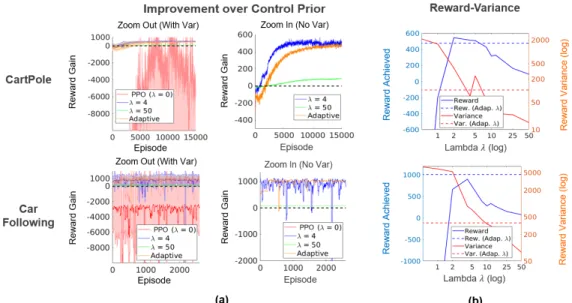
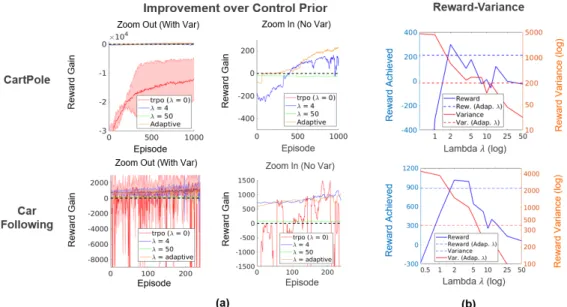
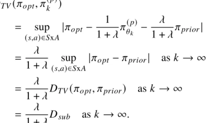
3.2) of the mixed policy derived from the policy gradient is reduced by a factor of (1+𝜆1 )2 when compared to the RL policy without precontrol. However, the mixed policy may introduce bias proportional to the sub-optimality of the prior control.
Control Theoretic Stability Guarantees
The dynamics of the system (3.24) can be expressed in terms of the linearization (3.25) plus a disturbance term as follows, The stability of the nonlinear system (3.26) under the mixed policy (3.3) can now be analyzed using Lyapunov theory [96].
Empirical Results
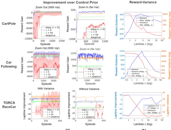
While Lemma 2 proved that the mixed controller (3.4) has the same optimal solution as the optimization problem (3.5), computational experiments using the loss in equation (3.5) found that the performance (i.e., the reward) is worse than CORE -RL and still had high variance. Performance is again based on the previous control, so any performance value above 0 represents an improvement over the previous control. Position (via GPS), speed and acceleration data were recorded from each of the cars, and the acceleration/deceleration of the 4𝑡 ℎ car in the chain was monitored.
Experimental data is divided into 10-second “episodes”. The episode data is shuffled and CORE-RL is applied six times with different random seeds (for several different ones). For each value of 𝜆, the algorithm is applied 5 times with different initializations and random seeds. Once again, Figure 3.4a shows that the adjusted controllers perform better on average than the basic RL algorithm and improve upon the previous controller.
Conclusion
Given a setC ∈ R𝑛defined by (2.7), the smooth functionℎ:R𝑛 →R is a discrete time-control barrier function (CBF) for dynamical system (4.1) if there exists𝜂 ∈ [0,1] such that for all𝑠𝑡 ∈𝐶,. It adjusts the gradient step sizes to ensure that the next parameter update falls within a "region of confidence". The code for these examples can be found at [2]. For the first policy iteration, the roll angle is maintained close to the edge of the safe area. The RL algorithm has suggested a bad control action so that the CBF controller provides the minimum intervention necessary to keep the system safe.
Robustness should always be at the expense of performance (e.g. the robot can reach the target faster if it doesn't care about collisions). The ratio between observed violations and expected violations was smaller than expected (i.e. the method was conservative), which is reassuring for safety. When the underlying distribution was Gaussian with uniform noise added (orange curve), the observed violations were much lower than the expected violations (i.e. the model was conservative).
Safe Reinforcement Learning through Control Barrier Functions . 47
Guiding Exploration in RL through CBFs
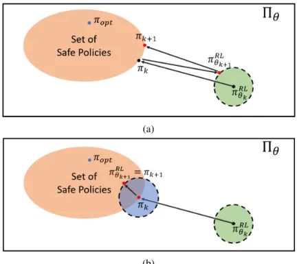
To show the implications of this difference, suppose the policy gradient (4.12) is used to update the RL policy at each iteration while using the policy (4.4). To account for the distortion in the policy gradient, inspired by (4.12), let us define the following guided policy. Using this policy (as opposed to the policy in (4.4)), the following difference can be defined at each iteration.
Using the policy𝜋𝑘(𝑠) from (4.14), if there exists a solution to the problem (4.16) such that𝜖𝑚 𝑎𝑥 =0, then the safe set Cis is forward invariant with probability (1− 𝛿). Moreover, if one uses TRPO for the RL algorithm, then the guided RL policy is 𝜋. 𝑎|𝑠)from(4.14) obtains the performance guarantee𝐽(𝜋. If there is no uncertainty in the dynamics, then the security is guaranteed with probability 1. Note that the performance guarantee in Theorem 3 is for policy 𝜋. 𝑎|𝑠), which is not the implemented policy,𝜋𝑘(𝑎|𝑠).
Simulation Results: RL-CBF
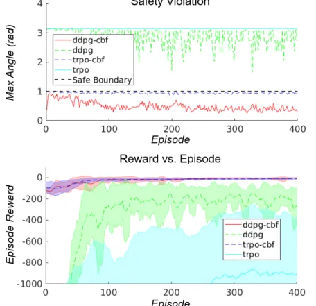
Bottom) Comparison of accumulated reward from the inverted pendulum problem using TRPO, DDPG, TRPO-CBF and DDPG-CBF. The left graph and the right graph show results from TRPO-CBF and DDPG-CBF, respectively. From Figure 4.5, it is shown that there were no safety violations between machines during the simulated experiments when using any of the RL-CBF controllers.
Furthermore, as seen in Figure 4.5, TRPO-CBF learns faster and performs better than TRPO (DDPG-CBF also outperforms DDPG, although neither algorithm converged on a high-performance controller in the experiments). Although DDPG and DDPG-CBF failed to converge on a good policy, Figure 4.5 shows that DDPG-CBF (and TRPO-CBF) always maintained a secure controller. Bottom) Comparison of reward across multiple episodes of car-following problem with TRPO, TRPO-CBF and DDPG-CBF (DDPG is excluded because it shows very poor performance).
Robust Safety in Uncertain, Multi-Agent Interactions
Inspired by the multi-agent CBF proposed in [27] (discussed in Section 2.2), consider the following CBF for the discrete time system, . However, recall that the dynamical system has relative degree 2, which allows us to derive the following bound. The following lemma allows us to use CBC bound (4.40) to obtain safety guarantees under polytopic uncertainties.
Then the action,𝑢, obtained from the solution of the following optimization problem (4.42) strongly satisfies the CBC condition (4.38) (i.e. it makes setCforward invariant). Therefore, the following section examines the problem of learning accurate polytopic uncertainty bounds𝑑in an online manner. High Confidence Security Guarantee: Combining the uncertainty associated with the previous result encapsulated in Lemma 5 leads to the main result, summarized in the following theorem.
Simulation Results: Multi-agent CBF
For fair comparison, robust and nominal CBFs were tested on the same 1000 random trials. The closer the steady-state CBF is to the nominal CBF, the less conservatism is introduced by the uncertainty prediction. However, the results in Table 4.1 show that strong CBF introduces only a slight conservatism, as the collision difference (in cases where CBF was active) was very similar when using strong CBF vs.
The code for the implementation of the robust multi-agent CBF in the simulated environment can be found online [3].
Conclusion
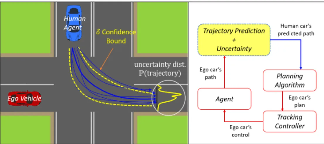
However, it is crucial to note that all guarantees of safety depend on accurate models of the uncertainty. In this example, the red car must account for the blue car's trajectory—and its uncertainty—in its plan to get safely through the intersection. To demonstrate its performance, quantile boundaries are calculated for each trajectory in the test set of the HighD dataset using the corresponding scenarios from the training set.
The core of the security guarantees provided by the proposed framework derive from behavioral contracts. Therefore, a "1" in a given voxel means that the agent's position was within that grid cell at that moment in the future. Can autonomous vehicles identify, recover from and adapt to distribution shifts?” In: International Conference on Machine Learning.
Safety Guarantees under Learned Models of Human Behavior
Accuracy of Learned Models of Human Uncertainty
Using the highD dataset and treating the trajectories in the training set as observed samples, high confidence bounds (calculated as the convex hull of the training trajectories) were obtained such that new trajectories should lie within these bounds with probability at least 1−𝛿. For example, Figure 5.6 shows the predicted confidence limits for the driving case; the scenario optimization approach predicts that each car's future track should fall within the blue confidence limits at 2.4.6 seconds in the future with 97.1% probability. The position history of the car is shown in red circles, and the training data is taken from the equivalent scenarios in the highD dataset.
Calculations show that there is a 97.1% probability that a new trajectory will fall within the blue confidence limits 2, 4, and 6 seconds into the future. To test the accuracy of the calculated confidence limits, I examined how often the trajectories in the test set actually remained within those limits in the highD data set (over a 2 second horizon). For example, if a new point falls in the interval covered by the blue bar, it can be classified as coming from mode 1 with confidence 𝛿≤ 10−8.
Guaranteeing Safety among Humans through Behavioral Contracts . 94
Conclusion
Future Work