Roads to Riches:

(1)

Vanderbilt University

Roads to Riches:

A Study of TIGER Grants

Senior Honors Thesis April 17, 2019

Author:

Jeffrey Jou

Advisor:

Dr. Matthew

Zaragoza-Watkins

(2)

Abstract

This paper exploits quasi-random variation through the Transportation Infrastructure Gen- erating Economic Recovery (TIGER) federal discretionary grants program to implement an instrumental variable and fixed effects difference-in-differences research design to estimate the impact of fiscal infrastructure investment on economic growth. The study finds that federal funds stimulate state and local general expenditures without causing substitutionary effects on state and local transportation spending. The introduction of federal grants to Metropolitan Statistical Areas generates a cumulative increase of more than 20 percent in real GDP across seven years.

(3)

This project has been one of the most energizing academic experiences I have ever had, and I owe its success to the help of many people. I would like to express my sincere gratitude to my advisor, Dr. Matthew Zaragoza-Watkins for his continuous support, patience, motivation, and immense knowledge. I am extremely fortunate and grateful for his guidance in all the time of research and writing of this thesis. His mentorship and teachings extend well beyond the pages of this paper. I would also like to thank Dr. Mario Crucini, for his role as both program director and second reader, generously giving his time to teach me new ideas week after week. Without their insightful comments and constant encouragement, this thesis would not have been possible.

(5)

I. Introduction

In the United States, state and federal governments spend more than $400 billion on transportation infrastructure each year. However, the stock of infrastructure has steadily declined over the last four decades due to deferred maintenance and underinvestment. As a result, over the same time period, productivity growth among private firms has also declined, likely due to degraded public inputs to productivity (Foster et. al. 2016). The macroeconomic effects of adequate levels of investment and timely maintenance show that an additional $12 billion spent on road maintenance is predicted to have saved $45 billion in reconstruction efforts – more than 10 percent of total infrastructure spending (Rioja 2001).

Public infrastructure is an important field of study, because these investments provide critical inputs for aggregate productivity. A temporary surge in public expenditures has been estimated to bring about a multiple expansion of output, to the magnitude of four to seven times as large as public-sector outlays (Aschauer 1989).

While results from past research suggest that government infrastructure spending can lead to positive economic growth, the magnitude of these effects is often debated. In areas where significant public infrastructure already exists within the economy, the benefits of new infrastructure construction are far more ambiguous (Talley 1996). Moreover, while public expenditures have a positive outcome on GDP, when used in excess, these expenditures have detrimental effects. Excessive amounts of transportation investment lead to unproductive spending as a result of diminishing marginal returns (Devarajan et. al. 1996). As stated before, public transportation infrastructure is an important field of study as it provides critical inputs for productivity. Infrastructure investment has been found to not only spur economic growth by giving access to previously underdeveloped natural resources, but also supplying ports and roads to transport goods as well as decreasing commuting times and costs for local residents (Talley 1996).

The wide discrepancies among the findings and results can be attributed to underlying econometric problems. The primary obstacle to estimating the causal impact of public infrastructure is that government spending is innately endogenous with past, current, and expected future private economic activity. For example, economic growth is closely correlated

(6)

with increased demand for freight and passenger traffic (Banister and Berechman 2001). As a result, past research designs are likely to suffer from endogeneity and omitted variable bias, leading to distorted estimates (Eisner 1991). The issue manifests itself in the direction of causality: whether transportation investment drives economic growth or whether increased economic activity promotes the need for more transportation and public investment.

Although the effects of public transportation spending have been a well-researched field of study, the findings are inconclusive, motivating this paper to formally quantify the effects of transportation infrastructure investment on economic growth. This paper departs from existing literature in two important ways. First, prior research on the effect of economic development and fiscal structure has relied heavily on cross-sectional or time-series variation (Easterly and Rebelo 1993). Instead, this paper employs panel data and a fixed-effects difference-in-differences design to eliminate omitted variable bias that may influence estimates. Second, the question of directionality has not been adequately addressed in prior studies. Hence, this paper utilizes the introduction of the Transportation Investment Gen- erating Economic Recovery (TIGER) discretionary grants program as an instrument aimed at avoiding endogeneity. TIGER grants serve as an instrument on local county government general and transit expenditures to predict the overall change in spending as a result of a federal injection of capital. This instrumental variable approach in conjunction with a fixed- effects difference-in-differences methodology will be implemented to isolate the treatment effects and provide unbiased estimates of the effects of public infrastructure spending on Metropolitan Statistical Area (MSA) real GDP. Results show that MSA real GDP increases by more than 20 percent, cumulatively, over the course of seven years after the initial grant was awarded to a county within the MSA.

The findings from this paper have both practical policy implications as well as research interest for further studies in transportation infrastructure and fiscal investment. The results offer a quantified effect for the impact of infrastructure spending on stimulating economic growth. The hope is that a closer and more in-depth understanding of the tangible costs and benefits for fiscal infrastructure investment will shape future policy initiatives. Moreover, the results offer an insight on the impact of fiscal spending during economic recessions. A positive result in the association between infrastructure spending and economic growth may

(7)

provide a solution to dampening the effects of future economic recessions. This research also provides a new empirical framework for investigating infrastructure spending and contributes to a growing body of literature surrounding proactive government spending.

II. Transportation Infrastructure Funding and TIGER Grants

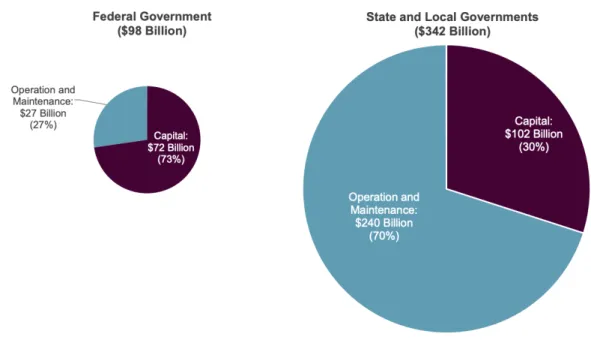
Federal grants have accounted for nearly 40 percent of all transportation and water infrastructure funding between 2001 and 2016. Beyond acting as a funding source, the federal government also spends an average of almost $100 billion annually. State and local governments invest nearly three times that amount at $330 billion per year in transit infrastructure.

The large disparity in funding levels across the different types of governments reflects the compositional differences in how the dollars are used. In 2017, 70 percent of state and local government funds were invested in operation and maintenance of infrastructure, while 30 percent were put into new projects. The opposite holds true for federal funds. Nearly three-quarters of federal dollars were placed into building new infrastructure projects while the remaining quarter of funds was used to cover operation and maintenance expenses.

Figure I: Shares of Public Spending by Level of Government

Notes: Decomposition of transit fund usage by federal and state and local governments.

Expenditure data is from 2017.

Source: Congressional Budget Office.

(8)

Since federal dollars play a large role in financing new infrastructure projects, a critical component of the American Recovery and Reinvestment Act (ARRA) included the TIGER grant program for the United States Department of Transportation (DOT) to support and facilitate state and local infrastructure projects. Since its inception in 2009, the TIGER program has provided nearly $5.6 billion through nine rounds of national infrastructure investments. TIGER grants served as targeted investments for local communities aimed at increasing safety, creating jobs, and modernizing the county’s infrastructure by providing funding for capital investments to improve the nation’s highway, bridge public transportation, rail, and port infrastructure. The program has provided funding to 463 projects across all 50 states, the District of Columbia, Puerto Rico, Guam, and the Virgin Islands. Each round reserves the requirement to award at least 20 percent of funding for projects in rural areas.

Given the context of the Great Recession immediately preceding the introduction of ARRA and the subsequent role of proactive fiscal spending on transportation infrastructure investment through TIGER, a set of important questions arises. First, this study is interested in understanding the impact of federal dollars in dampening the detrimental effects of the recession on affected counties. While theoretical frameworks suggest that federal investment can spur spending and pull economies out of recessionary periods, there is little consensus on the quantified effects of fiscal transportation infrastructure investment on economic growth.

Second, this paper looks to understand the complementary or substitutionary effect of federal dollars. The injection of federal funds may cause state and local governments to divert funds away from planned infrastructure investment and into other areas and public goods. It is imperative to understand if fiscal expenditures amplify spending at the county level or if these expenditures cause substitutionary effects, ultimately leading to no significant net changes to economic growth.

II.A. TIGER Grant Selection Process

The criteria used to select the top projects for these grants aligned with the Obama Administration’s Infrastructure principles of supporting economic vitality and promoting transit innovation. The primary selection criteria for TIGER awards included considera- tions for (1) Safety, (2) State of Good Repair, (3) Economic Competitiveness, (4) Quality

(9)

of Life, and (5) Environmental Stability. Safety refers to improvements in the safety of U.S.

transportation facilities and systems. State of Good Repair pertains to improving the condi- tion of existing transportation facilities and systems. Economic Competitiveness deals with improving the long-term efficiency of using the transportation network in the movement of workers or goods. TIGER grants placed specific emphasis on cost reduction and increased productivity for cargo transportation. Quality of Life considers increased transportation choices and access for people and communities. Environmental Stability underscores the im- provement of energy efficiency and reduction of greenhouse gas emissions. Primary criteria also included an aspect of job creation and economic stimulus.

Moreover, the Notice of Funding Opportunity (NOFO) for TIGER listed secondary criteria consisting of two main categories: Innovation and Partnerships. Innovation is scored based on new methods, including project financing, to address TIGER’s long-term strate- gic outcomes. Partnerships considers applicant partners with stakeholders as a means of leveraging alternative private and public funds. As a funding structure, TIGER utilized a competitive, merit-based process to allocate and distribute the funds. Applicants were encouraged to implement the suggested benefit-cost analysis (BCA) as a method of under- scoring the project’s merit. Applications were then scored based on the criteria, enabling the DOT to examine each project based on their merits and ensure that taxpayers received the highest return on invested capital. The likelihood of positive net benefits and BCA quality had significant impact on determining the success of the application, especially in the earlier rounds. However, a large number of projects with lower quality BCAs received grants in later rounds, suggesting that the influence of these variables diminished over time.

III. Data Overview and Summary Statistics

To implement the estimation strategy, one needs datasets for state and local expenditures as well as information on the counties that applied and were accepted for TIGER grants. For the output variable, an additional dataset tracking real GDP over time is also required. Other datasets, such as employment statistics, offer valuable observable control variables. State and local expenditure data were aggregated by MSA to match the real GDP estimates.

(10)

III.A. Individual County Finance Data

The primary source of data used in this project comes from the Census Bureau’s database on State and Local Government Finances across a fifteen-year time frame between 2001 to 2015. Since TIGER grants was introduced in 2009 and awarded through 2017, data points observed before the implementation of the grants program will be used to assess if pre- TIGER trends differ substantially across to the main sources of identifying variation. The dataset provides individual local government finances for counties in categories including highway infrastructure investment, secondary education fund, and hospital expenditures. In total, the historical finance database includes 553 variables consisting of 121 revenue items, 254 expenditure items, 134 debt items (issued, retired, and outstanding), and 20 cash and securities items. In addition, the dataset provides 24 general reference variables such as population, school district enrollment, and census region codes. A total of 580,819 observations were recorded during this time period. These observations consist of all governments within the geographic area of each state, such as school districts and special districts. While the dataset is fairly comprehensive, the dataset contains nearly 45,000 blank records, 89 percent of which consist of census of governments and 92 percent are special districts.

III.B. TIGER Grants

A secondary dataset consisting of the universe of TIGER grant applications for funding cycles between 2009 to 2017 is used in conjunction with the individual county finance data to predict the overall change in spending as a result of federal capital injections. The eligibility requirements of TIGER allow project sponsors at the state and local levels to obtain funding for multi-modal, multi-jurisdictional projects that are more difficult to support through tra- ditional Department of Transportation programs. Information on each application includes project name, applicant county, TIGER round, project type, project description, funding amount, and approximate latitudinal and longitudinal coordinates for the project. Out of the 7,306 applications submitted, 463 projects received funding, a 6.3 percent acceptance rate. Matching TIGER information to county spending creates a panel dataset of treated and untreated counties that form the foundation of the research design. Currently, counties that received funding in the final two rounds of TIGER in 2016 and 2017 do not have cor-

(11)

responding individual finance data. As such, the combined panel dataset ranges from 2001 to 2015. As more state and local government expenditure data becomes available, counties awarded in the final years will be added into the dataset in a potential revisit of this research methodology and paper. The program rounds were assigned roman numerals (I-IX) corresponding to the fiscal year that the grants were awarded. Starting in its second year, the TIGER program featured a new Planning Grant category in which 33 planning projects were funded. TIGER grants were matched to the awarded county from the individual finance dataset and then aggregated to MSAs. A detailed round-by-round breakdown of awarded grants is shown below:

Round # of capital projects funded # of planning projects funded

I 51 -

II 42 33

III 46 -

IV 47 -

V 52 -

VI 41 31

VII 39 -

VIII 40 -

IX 41 -

Total 399 64

Source: DOT.

III.C. Real GDP by Metropolitan Statistical Area

The real GDP estimates provided by the Bureau of Economic Analysis (BEA) consist of observations aggregated by MSA by year. Each year contains estimates for 398 MSAs between 2001 and 2016. These data provide observations that link TIGER grants to a relevant output variable. Together, these datasets give a causal connection between treatment assignment and economic growth.

One limitation to the BEA data is that it is only disaggregated to the MSA level. Since

(12)

MSA data excludes certain rural areas from its collection methodology – which account for 20 percent of awarded grants per year – a fraction of the total projects is lost through this aggregation process. On the other hand, this aggregation captures local spillover effects to MSAs, so the bias of using MSAs as opposed to counties is theoretically ambiguous. Of the total 463 grants that were awarded, only 312 grants were to counties within MSAs. Similarly, out of 7,306 total applications, only 7,105 were from counties in MSAs. Although the BEA released a comprehensive dataset of county level GDP estimates in December 2018, the data only consist of observations from 2012 to 2015. As a result, the county level observations do not span the entirety of the pre- and post-treatment period and cannot give valid comparisons between counties. A potential revisit of this research design in the future may yield more precise estimates if a larger dataset is published by the BEA in forthcoming years.

III.D. Employment Statistics

The Quarterly Census of Employment and Wages (QCEW) provides relevant, annual employment statistics for counties across the United States. These statistics provide useful observable characteristics and are valuable in determining valid MSA counterfactuals for comparison. The QCEW consists of five annual variables: average establishment count, average employment, total wages, average weekly wage, and average pay.

III.E. Baseline MSA Characteristics

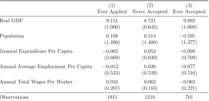
Table I presents the characteristics of the data categorized by application and acceptance status of the MSA. Observations were matched using propensity scores in order to identify valid counterfactuals. When comparing Columns (2) and (3), it is immediately clear that TIGER grants were generally awarded to MSAs with poorer economic outlooks.

On average, treated MSAs were shrinking in population size and experiencing reductions in general expenditures per capita. Furthermore, wages were declining at a faster rate than employment, signaling that, on average, economic conditions in these MSAs were deterio- rating. MSAs that did not receive federal funds underwent the opposite effect. Annual total wages outpaced average employment while population and general expenditure per capita grew at a steady rate.

(13)

Table I: Summary Statistics: Pre-TIGER Grant Introduction

(1) (2) (3)

Ever Applied Never Accepted Ever Accepted

Real GDP 9.151 8.721 9.893

(1.000) (0.645) (1.069)

Population 0.108 0.514 −0.595

(1.490) (1.400) (1.377)

General Expenditure Per Capita −0.002 0.053 −0.098

(0.669) (0.639) (0.709)

Annual Average Employment Per Capita −0.012 0.026 −0.077

(0.533) (0.539) (0.516)

Annual Total Wages Per Worker 0.016 0.062 −0.063

(0.207) (0.183) (0.221)

Observations 1911 1210 701

Notes: Summary statistics in the pre-treatment period of MSAs that applied at least once during the TIGER grant lifespan. Columns (2) and (3) represent sample statistics of MSAs that received no grants and at least one grant, respectively. Real GDP is reported in log form. Population, general expenditure per capita, annual average employment per capita, and annual total wages per worker averages estimated using log first differences.

Standard deviations in parenthesis.

Source: BEA, QCEW.

Given the Great Recession in 2008 that immediately preceded the introduction of the TIGER grants program, this result is not surprising. While the financial crisis impacted all MSAs in the United States, MSAs on a slower growth trajectory may have been dispropor- tionately affected by the recession. As such, TIGER dollars were funneled directly to MSAs that were on a downward economic trend beforehand in order to prop up economic growth and reduce the negative effects of the macroeconomic shock.

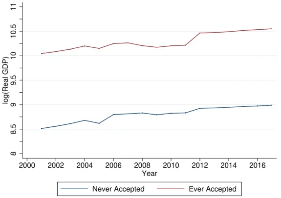
Figure II shows a line graph of average annual log(real GDP) for MSAs that applied but did not receive TIGER funding and MSAs that applied and did receive TIGER funding at least once during the program’s lifespan. The figure charts the progression throughout the pre- and post-treatment period. It is evident in the figure that while the “never accepted”

and “ever accepted” group differ in log(real GDP) levels, the two groups move in parallel during the pre-treatment period. In the post-treatment period, the “ever accepted” group

(14)

exhibits a larger jump in log(real GDP) between 2011 and 2012 as compared to the “never accepted” group before returning to parallel movements in the following years.

Figure II: MSA Real GDP by Treatment Status

88.599.51010.511log(Real GDP)

2000 2002 2004 2006 2008 2010 2012 2014 2016 Year

Never Accepted Ever Accepted

Notes: Plotted are the time-series average of MSA log(real GDP) by year from 2001 to 2016. Points estimates calculated using the mean log(real GDP) of MSAs by treatment status. “Ever accepted” group consists of all MSAs that applied and received at least one TIGER grant. “Never accepted” group composed of all MSAs that applied but did not receive any TIGER funding.

Source: BEA, DOT.

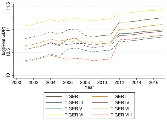
Figure III charts the changes in average annual log(real GDP) for the individual round- by-round cohorts of accepted MSAs. There is some variation in the trend lines between the cohorts during the pre-treatment period; however, all cohorts experience the same increase in log(real GDP) between 2011 and 2012, coinciding with the official end of the 2008 recession.

Following this surge, all cohorts move in parallel for the remaining years of the post-treatment period.

(15)

Figure III: MSA Real GDP by Year Cohort

1010.51111.5log(Real GDP)

2000 2002 2004 2006 2008 2010 2012 2014 2016 Year

TIGER I TIGER II

TIGER III TIGER IV

TIGER V TIGER VI

TIGER VII TIGER VIII

Notes: Plotted are the time-series average log(real GDP) of treated MSAs by year.

MSAs are separated into respective cohorts depending on TIGER round funding. Color coded dotted lines represent the corresponding pre-treatment period to the solid line post- treatment interval. TIGER IX is omitted from the figure due to incomplete data in MSA real GDP for year 2017 at the time of the study.

Source: BEA, DOT.

IV. TIGER Grants as a Research Design

Credible estimates of the effect of transportation infrastructure investment on economic growth requires the identification of a group of counties that are similar to those that received TIGER funding in observable and unobservable characteristics. Due to the innate endogeneity of infrastructure investment and economic growth, a na¨ıve comparison of real GDP growth rates between control and treatment groups is likely to yield biased results.

Fortunately, the quasi-random variation inherent in the dispersal of TIGER grants provides a solution to this identification problem.

TIGER grants vary over both time and space. Since only a fraction of applicants received funding in any given year, it is possible to estimate models that include control variables

(16)

that account for nationwide macroeconomic shocks to economic growth. Similarly, temporal variation exists from counties that received funding in different years across the project’s implementation, allowing for pre- and post-treatment period comparisons within counties.

As a result, any time-invariant unobservable characteristics can be controlled for through a time fixed-effects variable. The inclusion of county-specific and time-specific fixed effects variables motivates the usage of a fixed-effects difference-in-differences (DD-FE) research design to estimate the treatment effect.

In light of the differences in infrastructure funding sources detailed in the introduction, state and local governments are not prohibited from adding additional dollars onto federal grants. As such, the research design relies on not only comparing counties that did and did not receive TIGER grants, but also predicting the overall change in transit expenditures, prompting the usage of an instrumental variables (IV) design. TIGER grants serve as both the treatment assignment and the instrument in order to predict the total spending change in state and local governments. Since treatment assignment is not as good as random due to the merit-based selection process for TIGER grants, the DD-FE methodology will control for initial and inherent differences between counties that did and did not receive grant money.

Furthermore, since TIGER grants were awarded across multiple rounds between 2009 and 2017, the research design must reflect the fact that county economies may be on different growth patterns as a result of receiving the grants in earlier rounds. This issue motivates the usage of an event study difference-in-differences methodology. Using this methodology, observations in the datasets are indexed by the number of years pre- or post-treatment assignment. The event study design allows for uniform comparison across time.

Last, given the differences in observable characteristics between untreated and treated MSAs, there is reason to believe that certain MSAs are not valid counterfactual comparisons.

To address this issue, the paper employs propensity score matching in order to restrict the sample distribution to the overlapping region. This process ensures only MSAs that share the same propensity to be awarded federal funding are compared against one another in order to provide a more precise estimate of the treatment effect.

(17)

V. Measurement Framework

To effectively model this discretionary grant program, let Pre Treat be an indicator variable equal to 1 for observations before the MSA received TIGER grant funding and Post Treat be an indicator for observations after the MSA received federal capital. Year c is indexed to the MSA specific treatment year. Pre-treatment period includes n years prior to the year immediately preceding the treatment year c. Similarly, post-treatment years consist ofn years after the treatment year c, inclusive. Coefficients for both indicator variables represent a vector of coefficients designed to estimate the effect of the predicted change in general expenditures on MSA real GDP, forming the basis for the following DD-FE specification:

Y_it =α+

n

X

t=c−1

β_tPre Treat+

n

X

t=c−1

γ_tPost Treat +X_i+φ_i+ζ_t+_it (1)

where an outcome Y_it (i.e., real GDP) in the MSA i at time period t is regressed on the event study methodology for both pre- and post-treatment periods and a series of control variables. Yeart is indexed by the number of years before or after treatment yearc. Control variables consist of MSA specific time trends X_i; a set of MSA fixed effects φ_i that control for unobservable characteristics associated with MSA i that do not vary with time; and year fixed effects ζ_t to control for any unobservable characteristics that affect all counties simultaneously at timet. The error term,ε_it, represents unobservable determinants assumed to be uncorrelated with the regressor of interest.

The identifying assumption in this model is that trends between treatment and control groups are common throughout time. While the baseline MSA characteristics show that the two groups are on different growth trajectories during the pre-treatment period, a violation of the underlying common trends assumption, the growth trends are persistent throughout time allowing for valid comparisons. Potential detriments to the research design come from areas consistent with prior methodologies. Although this approach attempts to limit the effect of omitted variables bias on estimates, there is still the possibility that other conflating, exogenous sources driving economic growth in MSAs.

(18)

VI. Results

The results are presented in the following subsections. The section begins by examining the effect of federal funding on state and local government expenditures. As stated before, this study is interested in exploring the substitutionary and complementary effect of federal dollars. Therefore, output variables consist of both general and transit expenditures. The section continues by reporting the effect of TIGER grants on MSA real GDP. The final subsection offers various robustness checks on the results.

VI.A. Federal Funding Leads to Increase in General Expenditures

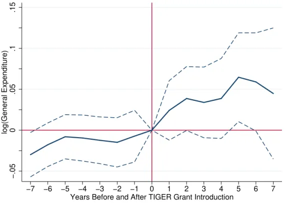
Economic intuition suggests that counties that receive an increased amount of federal funding will spend more than their non-funded counterparts. The findings in this study substantiate this claim. Column (2) of Table II shows the annual cumulative change in general expenditures for treated MSAs compared to control group counterfactuals. Immediately after receiving TIGER funding, treated MSAs exhibited an increase in general expenditures.

In the short-run, TIGER grants spurred an increase in general spending, peaking in year five at 6.5 percent. Over the lifetime of the program, this amplified investment diminished to a cumulative increase of 4.5 percent in state and local general expenditures after seven years.

Figure IV plots the event-time coefficients using average MSA log(state and local general expenditures) as the dependent variable. The plotted coefficients represent the time path of general expenditures in MSAs that received TIGER funding conditional on MSA specific and time specific fixed effects. There are two important features in Figure IV. First, the pre- treatment period trend line remains largely flat with no statistical significance away from 0.

This observation provides an important test to the validity of the identifying assumption.

Specifically, trends in outcomes across comparison groups evolve smoothly except for the change in federal funding. The second important feature of Figure IV is the post-treatment period deviation. Following the first year that TIGER grants were introduced, state and local government expenditures in treated MSAs began to increase, reaching a maximum cumulative increase of 6.5 percent after five years, as compared to counterfactual MSAs.

Although this amplifying effect gradually declines after the year five, total cumulative net changes are positive, with an overall expansion of 4.5 percent in general expenditures.

(19)

Figure IV: State and Local General Expenditure before and after TIGER Grants

−.050.05.1.15log(General Expenditure)

−7 −6 −5 −4 −3 −2 −1 0 1 2 3 4 5 6 7

Years Before and After TIGER Grant Introduction

Notes: Plotted are the event-time coefficient estimates from equation (1), where the dependent variable consists of log(state and local government general expenditures) in MSA i by year t. The regression model controls for MSA specific FE, time specific FE, and MSA-specific time trends The year prior to TIGER funding corresponds to year 0 in the figure. The dashed lines represent 95% confidence intervals.

Source: Census, DOT

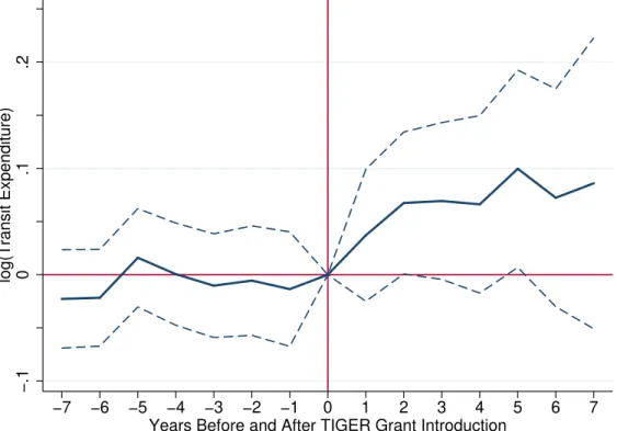
An important corollary to investigate is the effect of increased general expenditures on transit investment. Column (3) displays the cumulative annual change in state and local transportation expenditures. Since transit spending in the post-treatment period includes the injected federal funds, no statistically significant change from the pre-treatment period would suggest that state and local governments are maintaining the same level of transit spending as prior to receiving TIGER grant money. Instead, federal funds act to loosen budget constraints on state and local governments, allowing them to divert the additional funds away from planned transit outlays in favor of other public goods. While there are only two periods of statistical significance for the regression coefficients in Column (3), Figure V presents a different story. The plotted coefficients display a considerable upward trend in transit expenditures during the post-treatment period. This bump in spending likely reflects

(20)

the addition of federal funds, suggesting that there is no substantial substitutionary effect.

In this case, the lack of statistical significance is likely due to the fact that TIGER grants represented less than 1 percent of total transit investment. Had federal capital injections been of a larger magnitude in relation to total transit spending, the effect of TIGER dollars would have had a more pronounced increase to state and local government transportation expenditure.

Figure V: State and Local Transit Expenditure before and after TIGER Grants

−.10.1.2log(Transit Expenditure)

−7 −6 −5 −4 −3 −2 −1 0 1 2 3 4 5 6 7

Notes: Plotted are the event-time coefficient estimates from equation (1), where the dependent variable consists of log(state and local government transit expenditures) in MSA i by year t. The regression model controls for MSA specific FE, time specific FE, and MSA-specific time trends. The year prior to TIGER funding corresponds to year 0 in the figure. The dashed lines represent 95% confidence intervals.

Source: Census, DOT

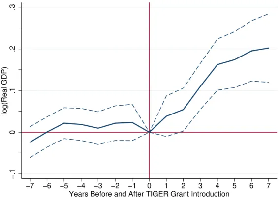
VI.B. Real GDP Expansion in Treated MSAs

While an increase in state and local general expenditures affirms past economic theories, this study is primarily interested in how increases in investment impacts economic growth.

Column (1) of Table II shows the compounded effects on MSA real GDP. Two years after

(21)

receiving TIGER funding, MSA real GDP increases by more than 5 percent and continues on this cumulative growth trajectory for future years.

Figure VI plots the event-time coefficients using average MSA log(real GDP) as the dependent variable. Coefficients in Figure VI follow the overall pattern of Figures IV and V in that the pre-treatment trend line remains flat while post-treatment coefficients exhibit a drastic deviation from 0. Another feature to note is the difference in growth rates between the short-run and long-run periods. In the four-year span immediately following the introduction of TIGER grants, log(real GDP) increases at a much faster rate than subsequent years. This pattern suggests that federal investment has a significant boost to economic growth in the short-run and gradually declines over time. Despite this change in rates, average MSA real GDP reaches cumulative levels 20.2 percent higher than its counterfactual after seven years.

Figure VI: MSA Real GDP before and after TIGER Grants

−.10.1.2.3log(Real GDP)

−7 −6 −5 −4 −3 −2 −1 0 1 2 3 4 5 6 7

Notes: Plotted are the event-time coefficient estimates from equation (1), where the dependent variable consists of log(real GDP) in MSA i by year t. The regression model controls for MSA specific FE, time specific FE, and MSA-specific time trends. The year prior to TIGER funding corresponds to year 0 in the figure. The dashed lines represent 95% confidence intervals.

Source: BEA, DOT

(22)

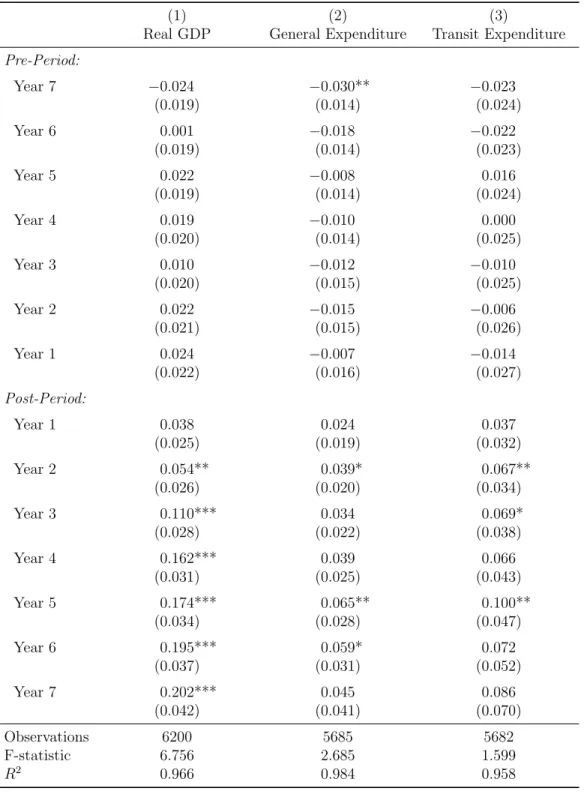
Table II: Fixed Effects Model on Real GDP, General and Transit Expenditure

(1) (2) (3)

Real GDP General Expenditure Transit Expenditure Pre-Period:

Year 7 −0.024 −0.030** −0.023

(0.019) (0.014) (0.024)

Year 6 0.001 −0.018 −0.022

(0.019) (0.014) (0.023)

Year 5 0.022 −0.008 0.016

(0.019) (0.014) (0.024)

Year 4 0.019 −0.010 0.000

(0.020) (0.014) (0.025)

Year 3 0.010 −0.012 −0.010

(0.020) (0.015) (0.025)

Year 2 0.022 −0.015 −0.006

(0.021) (0.015) (0.026)

Year 1 0.024 −0.007 −0.014

(0.022) (0.016) (0.027)

Post-Period:

Year 1 0.038 0.024 0.037

(0.025) (0.019) (0.032)

Year 2 0.054** 0.039* 0.067**

(0.026) (0.020) (0.034)

Year 3 0.110*** 0.034 0.069*

(0.028) (0.022) (0.038)

Year 4 0.162*** 0.039 0.066

(0.031) (0.025) (0.043)

Year 5 0.174*** 0.065** 0.100**

(0.034) (0.028) (0.047)

Year 6 0.195*** 0.059* 0.072

(0.037) (0.031) (0.052)

Year 7 0.202*** 0.045 0.086

(0.042) (0.041) (0.070)

F-statistic 6.756 2.685 1.599

R² 0.966 0.984 0.958

* p<0.1, ** p<0.05, *** p<0.01. Standard errors in parentheses.

Notes: This table reports regression coefficients from equation (1). Each column refers to a different regression with separate output variables. An observation is a MSA by year. All regressions control for MSA specific FE, time specific FE, and MSA-specific time trends. Sample is restricted to overlap using propensity score matching. Observations are indexed in the pre- and post-treatment period for every TIGER grant award year.

Source: BEA, Census.

(23)

VI.C. Robustness Check

One potential area of concern is that MSAs can apply and receive multiple grants throughout the program’s lifespan. Since TIGER grants set MSAs on higher growth trends, the treatment effect intensifies as MSAs receive more and more treatments. As a result, it may not be appropriate to include treated MSAs in the pre-treatment period after the MSA is initially awarded a grant. Tables and figures for this section are in the appendix.

To account for multiple treatments, the pre-treatment period is fixed to the first year of treatment for the MSA. Subsequent TIGER funds awarded to the MSA are captured only as variation in the post-treatment period, excluding them from the control group. The modified DD-FE specification is as follows:

Y_it=α+

n

X

t=I−1

β_tPre Treat +

n

X

t=c−1

γ_tPost Treat+X_i+φ_i+ζ_t+_it (2)

where an outcomeY_it (i.e., real GDP) in the MSAi at time periodt is regressed on the event study methodology for both pre- and post-treatment periods and a series of control variables.

Treatment year I represents the first year of treatment in MSA i. Yeart is indexed by the number of years before treatment yearI or after treatment year c. Control variables consist of MSA specific time trends X_i; a set of MSA fixed effects φ_i that control for unobservable characteristics associated with MSAi that do not vary with time; and year fixed effectsζ_tto control for any unobservable characteristics that affect all counties simultaneously at timet.

The error term, ε_it, represents unobservable determinants assumed to be uncorrelated with the regressor of interest.

The results find that the effect of transportation investment on MSA real GDP remain largely unchanged, while increases in general and transit expenditures are more pronounced.

Table III reports the findings of the revised model specification. Columns (2) and (3) show that TIGER funding had a slightly more prominent effect on state and local government general and transit expenditures as compared to the baseline model. The coefficient plots in Figures VII and VIII display the same pattern of persistent pre-treatment period trends followed by significant deviation in the post-treatment period. General expenditures showed

(24)

a cumulative increase of 6.7 percent after seven years while transit expenditures increased 9.1 percent over the same time period. Similarly, the effect on MSA real GDP is consistent.

Column (1) shows that treated MSAs experience a cumulative increase of 16.3 percent in real GDP over seven years. Moreover, Figure IX displays the same short-run effect followed by gradual decline as before.

After accounting for potential overlap in treated and control groups that may have upwardly biased the treatment effect, the overall effect of transit investment on MSA real GDP remains largely unchanged. This result addresses the primary concern of repeated treatments and sheds light on the validity of the research design.

VII. Discussion

A cursory overview of the coefficient plots and regression tables show that fiscal investment in infrastructure spurs substantial economic growth, offering empirical evidence to the claim initially brought forth by Aschauer (1989). A temporary surge in public expenditures does indeed generate a multiple expansion in economic growth. The magnitudes and dynam- ics of the estimates are larger than those of Duffy-Deno (1990), which uses OLS and 2SLS models to estimate the effect of public investment on personal income per capita. The OLS regression estimates that a 10 percent increase in public outlays increases personal income per capita by 0.37 percent, while 2SLS estimates a 1.1 percent increase. Moreover, the re- lationship between federal grants and public investment expenditures at the state and local government level is also consistent with the findings of Duffy-Deno. The 2SLS model found that a 10 percent increase in intergovernmental revenues per capita raises public investment expenditures by 0.25 percent in treated MSAs.

While the findings in this study are in line with prior research, this paper has furthered the field of study in public infrastructure investment by investigating the tradeoff effect between transit and general expenditures at the state and local government level. Some economists have hypothesized that depending on the investment preferences of individual counties, transit expenditures will be substituted away as a result of increased transit funding through federal grants. However, there is no evidence that MSAs divert funds away from planned infrastructure projects. Instead, state and local general expenditures increase across

(25)

all categories while transit expenditures remain largely unchanged. An important aspect to note are the matching requirements in transportation infrastructure. While there is no evidence that MSAs actively move funds out of transit investment after receiving an increase in intergovernmental revenue, this result may be driven by the fact that they are required to match federal funds with state and local dollars, rather than a strong preference for transit investment over other categories of spending. Apart from this finding, this paper has also given insight on the causal direction of infrastructure investment and economic growth.

Based on the various figures presented in previous sections, there is evidence that state and local government expenditures – both in transportation and in general – increase prior to the expansion in MSA real GDP. While others have theorized that MSAs with higher economic activity will require more capital investment, it is clear by the sequential timing of increased transit and general expenditures followed by heightened real GDP growth, that proactive government investment drives economic growth.

An important caveat to note in analyzing these results is the fact that TIGER grants were introduced and distributed as a reaction to the global financial crisis in 2008. More importantly, TIGER grants only represent a small portion (less than 1 percent) of the total ARRA stimulus bill. As such, other federal grants and reinvestment dollars may have in- fluenced and upwardly biased the effect that transportation infrastructure had on economic growth. That is to say, other aspects of fiscal spending aimed to counteract the detrimental effects of the recession may have also contemporaneously boosted economic growth. Simi- larly, the impact of transportation infrastructure may be overstated as a result of the Great Recession. Since counties and MSAs were already experiencing a slowdown in economic growth prior to the introduction of TIGER and ARRA, a portion of the stimulus may be attributed to recovery to pre-recession growth levels. As such, the same magnitude of economic growth may not be observed during non-recessionary time periods.

One aspect that warrants further investigation is the validity of TIGER grants as an instrument on general expenditures. The F-statistics reported in Tables II and III suggest that TIGER grants are a weak instrument, falling well short of the generally accepted threshold of 10. This result implies that while there is an observed increased in general expenditures, the change is largely unexplained by TIGER grants; instead, other covariates may have been the

(26)

primary drivers to this increase. As previously stated, the TIGER program only represented a small fraction of the overall stimulus bill. It is likely that MSAs that received TIGER grant funding also received federal investment in other forms under ARRA, boosting general expenditures.

However, the larger implication of fiscal spending still remains. While estimates may be slightly overstated due to other factors, the results of this study shed light on the effectiveness of fiscal stimulus. Neoclassical economic models have suggested the importance of federal spending in dampening the negative effects during economic downturns. The findings in this paper support those hypotheses, showing that increases in fiscal investment translate directly to increases in economic growth across the entire United States.

VIII. Conclusion

This paper makes two primary contributions to the existing literature surrounding the impact of transportation infrastructure investment on economic growth. First, the estimates document a quantified effect of infrastructure spending on real GDP. On average MSAs that received federal funding through TIGER grants experienced a cumulative increase of 20.2 percent on MSA real GDP. A 1 percent increase in federal transit infrastructure investment drives a 2.3 percent increase in MSA real GDP. Prior research focused on cross-sectional and time-series variation, whereas this study exploits quasi-random variation through the TIGER federal discretionary grants program. Panel data consisting of all MSAs in the United States across a fifteen-year timeframe from 2001 to 2016 allows for a fixed effects difference-in-differences research design. In turn, the estimated treatment effect is more precise than previous literature and offers a clearer insight to the efficacy of fiscal transportation infrastructure investment in stimulating economic growth.

Second, this paper examines the effect of federal funding on state and local expenditure preferences. The findings show that there is no evidence of substitutionary effects in state and local transit spending. Across the seven-year post-treatment time period, MSAs that received federal dollars exhibited an increase in total transit infrastructure amount invested, reflecting the injection of federal capital. Since the spending deviated from the pre-treatment period significantly, there is no evidence that state and local dollars were diverted away

(27)

from planned transit outlays. Instead, general expenditures, as a whole, increased in other categories of public goods.

Given the context of the Great Recession in 2008, the results from this study support arguments in favor of proactive government intervention as a method of revitalizing economic growth. MSA real GDP increases substantially as a result of fiscal capital injections.

These findings highlight the efficacy of fiscal investments in dampening the negative effects of adverse macroeconomic shocks, providing evidence of rapid short-run growth following increased investment in transportation infrastructure. The empirical approach presented in this paper could be applied to any number of areas concerning federal discretionary grants programs. The primary shortcoming to this study is the strength of TIGER grants as an instrument for general expenditures and real GDP. However, with the growing availability of post-recession data, future studies aimed at identifying stronger instruments should provide for a fruitful area of research.

(28)

Appendix

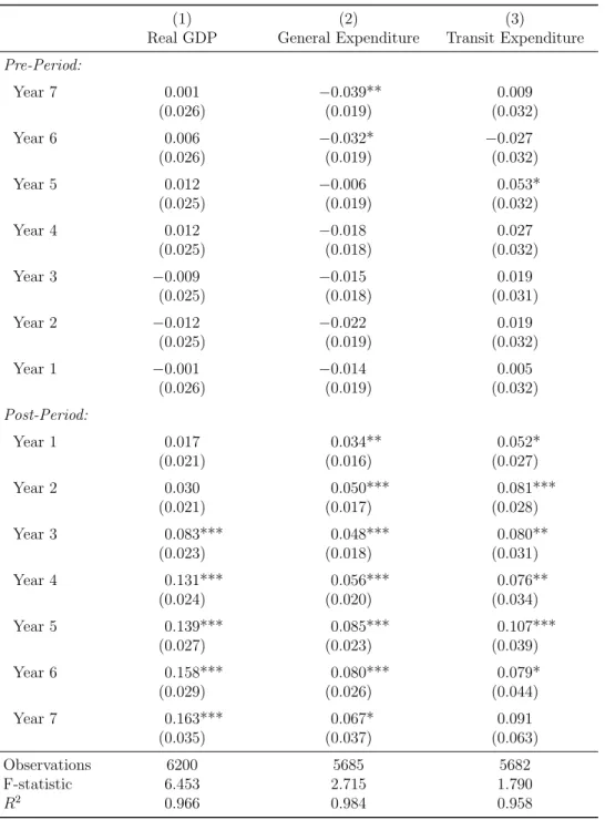
Table III: Fixed Effects Model on Real GDP, General and Transit Expenditure

(1) (2) (3)

Real GDP General Expenditure Transit Expenditure Pre-Period:

Year 7 0.001 −0.039** 0.009

(0.026) (0.019) (0.032)

Year 6 0.006 −0.032* −0.027

(0.026) (0.019) (0.032)

Year 5 0.012 −0.006 0.053*

(0.025) (0.019) (0.032)

Year 4 0.012 −0.018 0.027

(0.025) (0.018) (0.032)

Year 3 −0.009 −0.015 0.019

(0.025) (0.018) (0.031)

Year 2 −0.012 −0.022 0.019

(0.025) (0.019) (0.032)

Year 1 −0.001 −0.014 0.005

(0.026) (0.019) (0.032)

Post-Period:

Year 1 0.017 0.034** 0.052*

(0.021) (0.016) (0.027)

Year 2 0.030 0.050*** 0.081***

(0.021) (0.017) (0.028)

Year 3 0.083*** 0.048*** 0.080**

(0.023) (0.018) (0.031)

Year 4 0.131*** 0.056*** 0.076**

(0.024) (0.020) (0.034)

Year 5 0.139*** 0.085*** 0.107***

(0.027) (0.023) (0.039)

Year 6 0.158*** 0.080*** 0.079*

(0.029) (0.026) (0.044)

Year 7 0.163*** 0.067* 0.091

(0.035) (0.037) (0.063)

F-statistic 6.453 2.715 1.790

R² 0.966 0.984 0.958

* p<0.1, ** p<0.05, *** p<0.01. Standard errors in parentheses.

Notes: This table reports regression coefficients from equation (2). Each column refers to a different regression with separate output variables. An observation is a MSA by year. All regressions control for MSA specific FE, time specific FE, and MSA-specific time trends. Sample is restricted to overlap using propensity score matching. Observa- tions that received multiple treatments are only indexed in the post-treatment past the initial TIGER grant.

Source: BEA, Census.

(29)

Figure VII:State and Local General Expenditure before and after TIGER Grants

−.1−.050.05.1.15log(General Expenditure)

−7 −6 −5 −4 −3 −2 −1 0 1 2 3 4 5 6 7

Notes: Plotted are the event-time coefficient estimates from equation (2), where the dependent variable consists of log(state and local government expenditure) in MSAi by yeart. The regression model controls for MSA specific FE, time specific FE, and MSA- specific time trends. The year prior to TIGER funding corresponds to year 0 in the figure.

The dashed lines represent 95% confidence intervals.

Source: Census, DOT.

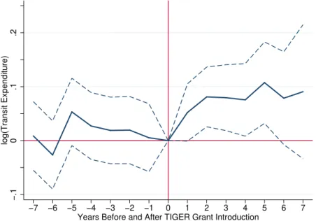
Figure VIII:State and Local Transit Expenditure before and after TIGER Grants

−.10.1.2log(Transit Expenditure)

−7 −6 −5 −4 −3 −2 −1 0 1 2 3 4 5 6 7

Notes: Plotted are the event-time coefficient estimates from equation (2), where the dependent variable consists of log(state and local government transit expenditure) in MSA i by yeart. The regression model controls for MSA specific FE, time specific FE, and MSA-specific time trends. The year prior to TIGER funding corresponds to year 0 in the figure. The dashed lines represent 95% confidence intervals.

Source: Census, DOT.

(30)

Figure IX:MSA Real GDP before and after TIGER Grants

−.10.1.2.3log(Real GDP)

−7 −6 −5 −4 −3 −2 −1 0 1 2 3 4 5 6 7

Notes: Plotted are the event-time coefficient estimates from equation (2), where the dependent variable consists of log(real GDP) in MSAi by yeart. The regression model controls for MSA specific FE, time specific FE, and MSA-specific time trends. The year prior to TIGER funding corresponds to year 0 in the figure. The dashed lines represent 95% confidence intervals.

Source: BEA, DOT.

(31)

References

Aschauer, David A., “Is Public Expenditure Productive?,” Journal of Monetary Eco- nomics, 1989, 23 (2), 177–200.

Banister, David and Yossi Berechman, “Transport Investment and the Promotion of Economic Growth,”Journal of Transport Geography, 2001,9 (3), 209–218.

Cashin, Paul, “Government Spending, Taxes, and Economic Growth,”International Mon- etary Fund, 1995, 42(2), 237–269.

Devarajan, Shantayanan, Vinaya Swaroop, and Heng fu Zou, “The Composition of Public Expenditure and Economic Growth,” Journal of Monetary Economics, 1996, 37 (2), 313–344.

Duffy-Deno, Kevin T. and Randall W. Eberts, “Public Infrastructure and Regional Economic Development: A Simultaneous Equations Approach,” Journal of Urban Eco- nomics, 1990, 30 (3), 329–343.

Easterly, William and Sergio Rebelo, “Fiscal Policy and Economic Growth: An Em- pirical Investigation,”Journal of Monetary Economics, 1993, 32(3), 417–458.

Eisner, Robert, “Infrastructure and Regional Economic Performance: Comment,” New England Economic Review, 1991.

Foster, Lucia, John Haltiwanger, and Chad Syverson, “The Slow Growth of New Plants: Learning about Demand?,”Economica, 2016, 83 (329), 91–129.

Homan, Astrid C., “Role of BCA in TIGER Grant Reviews: Common Errors and Influence on the Selection Process,”Journal of Benefit-Cost Analysis, 2013,5 (1).

, “Notice of Funding Opportunity (NOFO) of Transportation’s National Infrastructure In- vestments Under the Consolidated Appropriations Act,” Office of the Secretary of Trans- portation, 2017.

, “Public Spending on Transportation and Water Infrastructure, 1956 to 2017,” Congres- sional Budget Office, October 2018.

Rioja, Felix K., “Filling Potholes: Macroeconomic Effects of Maintenance Versus New Investments in Public Infrastructure,”Journal of Public Economics, 2003,87 (9-10).

Talley, Wayne, “Linkages Between Transportation Infrastructure Investment and Economic Production,” Logistics and Transportation Review, 1996,32 (1), 145.

Walker, W. Reed, “The Transitional Costs of Sectoral Reallocation: Evidence from the Clean Air Act and the Workforce,”The Quarterly Journal of Economics, November 2013, 128(4), 1787–1835.

Roads to Riches:

Vanderbilt University

Roads to Riches:

A Study of TIGER Grants

Senior Honors Thesis April 17, 2019

Author:

Jeffrey Jou

Advisor:

Dr. Matthew

Zaragoza-Watkins

Contents