STONE CENTER ON SOCIO-ECONOMIC INEQUALITY WORKING PAPER SERIES
No. 55
Intergenerational Mobility in Income and Consumption:
Evidence from Indonesia
Rafia Zafar
September 2022
Consumption: Evidence from Indonesia ∗
Rafia Zafar
†Abstract
This paper estimates absolute and relative intergenerational mobility for Indonesia.
My preferred estimates that address both measurement error bias and life-cycle bias show lower intergenerational mobility than standard estimates. I also examine absolute mobility, which separates upward mobility from downward mobility. At the bottom of both the income and consumption distribution, I find lower absolute intergenera- tional mobility compared to people at the top of the distribution. This paper makes a unique contribution to the literature by showing that household survey data on in- come and consumption can facilitate reliable estimates for intergenerational mobility in developing countries.
Keywords: Intergenerational Mobility, Measurement Error, Instrumental Variable JEL Classification: J62, I32
∗I am grateful to Subha Mani for her guidance. I would also like to thank Leslie McCall, Janet Gornick, Sophie Mitra and Andrew Simons for their feedback and input. This paper immensely benefited from feedback from seminar participants at Fordham University and Stone Center of Socio-Economic Inequality, and from conference participants at NYSEA (2018), SEA (2018), EEA (2019), NEUDC (2020). All errors are my own.
†Stone Center on Socio-Economic Inequality, CUNY, [email protected]
1
1 Introduction
Global economic growth and liberalization have reduced overall poverty but also increased inequality around the world (World Development Report, 2006). Through various mech- anisms, these high levels of inequality may reduce the ability of children born into poor households to escape poverty. This potential reduction in intergenerational mobility raises both economic and ethical concerns. Through misallocation of resources, inefficiencies, and ultimately lower economic output, lower intergenerational mobility not only compounds in- equality but also impacts economic growth.
The evidence on intergenerational mobility from developed countries is vast and growing (Bj¨orklund et al., 2012; Chetty, Hendren, Kline, & Saez, 2014; Chetty, Hendren, Kline, Saez,
& Turner, 2014; Corak & Heisz, 1999). The rise in inequality, especially in developed coun- tries, is mostly due to the divergence of income between the top 1 percent and the rest of the population. Although income in the middle of the distribution has stagnated across recent generations in some developed countries, wages for highly skilled workers have continued to grow (Chetty, Friedman, et al., 2017; Corak et al., 2014). Access to decades of reliable data on earnings, income, and taxes has allowed researchers to measure intergenerational mobility extensively in these countries. However, there is less evidence on this topic from developing countries (Narayan et al., 2018).
The need for further evidence stems from the fact that 80 percent of the world popula- tion lives in developing countries, where widening income inequality has heightened concerns about lower intergenerational mobility.1 Lower mobility in developing countries is mainly driven by unequal access to education and health care, as well as inefficient resource al- locations, all of which can impact lifetime earnings for individuals born into low-resource households. Crucial evidence on intergenerational mobility necessary to guide policy initia- tives in developing countries is very limited, with a few exceptions (Asadullah, 2012; Azam, 2016; Bevis & Villa, 2017; Fan et al., 2021).
The key challenge in developing countries has been data - we need reliable income data over many years and generations, but in developing countries, these data are rarely well maintained or readily available. Even if we have access to income data from tax records, concerns are further exacerbated by employment in the informal sector. For instance, ap- proximately 61 percent of the world’s population is employed in the informal sector (ILO Report, 2018) where no tax records are available. If we rely on tax records to estimate mobility, we will therefore lose information on many vulnerable groups. Appropriate data are available in some household surveys in the form of reported income, and more usefully, consumption expenditures, but the latter data have been underutilized.
Most previous studies of developing countries use data on education, occupation, or assets to estimate intergenerational mobility, with a few using earnings or income. For example,
12007 Human Development Report (HDR), United Nations Development Program, November 27, 2007, p. 25.
current evidence on intergenerational mobility in India, Bangladesh, and the Philippines shows lower mobility in these countries relative to higher-income countries. Asher et al.
(2017) found some gains in rank mobility in education for low-caste groups, but this gain disappears for Muslims in India. Bevis and Villa (2017) found a strong correlation between daughters’ and parents’ income and education in the Philippines. Asadullah (2012) esti- mated intergenerational persistence in wealth between father-son pairs in rural Bangladesh to be between 0.35 and 0.53, which suggests low intergenerational mobility there. A com- prehensive study by Grawe (2004) examined the father-son earnings data from the US, UK, Pakistan, Peru, Nepal, Malaysia, and Ecuador. He found significantly lower intergenera- tional mobility in developing countries. A recent paper by Fan et al. (2021) documented the rising intergenerational income persistence in China since 1970.
To fill the existing gap in the literature, in this paper I estimate intergenerational mobil- ity for Indonesia. Specifically, I combine rich data on income and consumption expenditures available from multiple waves of the Indonesian Family Life Survey to estimate intergen- erational mobility, addressing both attenuation bias and life-cycle bias in mobility. In my IV estimation strategy, I address attenuation bias by instrumenting income from one year for another year. To address both life-cycle bias and measurement error bias, my preferred estimates on intergenerational mobility use consumption expenditures, which captures a household’s long-run economic status more accurately. Consumption expenditure has also been a preferred measure for constructing poverty lines in developing countries, as it is often subject to much less measurement error than income (Ravallion, 2015). Importantly, this measure also captures the co-residence aspect of multi-generational households in developing countries. These are the households where multiple heads of family live in the same house, such as an adult son and his wife and children living with his parents or sharing a house with another brother and his family. Co-residence is an important potential source of economic mobility in developing countries, as multiple generations commonly live together under one roof and pool resources (Cameron & Cobb-Clark, 2008; LaFave & Thomas, 2017; Raut &
Tran, 2005). There are few studies on developed countries as well which rely on consump- tion expenditure data to estimate consumption inequality and intergenerational mobility.
Attanasio and Pistaferri (2016) and Charles et al. (2014) use a longitudinal panel survey to estimate consumption inequality and intergenerational correlations in consumption expen- ditures. Bruze (2018) use Danish expenditure survey to estimate intergenerational elasticity in consumption in Denmark.
In order to estimate intergenerational mobility, I construct parent-child pairs using five rounds of the Indonesian Family Life Survey (IFLS), collected over 25 years. I next estimate absolute and relative mobility using both income and per capita consumption expenditures.
To address inequalities that vary across generations, I also present rank-rank estimates by controlling for varying standard deviations in income for both generations.
Overall, I find: (a) an uncorrected, baseline coefficient of 0.08 using reported income, which suggests higher income mobility in Indonesia than in developed countries; (b) a higher coefficient (0.45) and thus lower mobility when reported income is corrected for measure- ment error bias using an instrumental variable specification; and (c) a coefficient of 0.25
when using per capita consumption expenditures as a measure of permanent income. I find that mobility estimates are sensitive to measurement error bias, suggesting that previous estimates may be severely overestimating intergenerational mobility (that is, finding lower coefficients of intergenerational elasticity). My preferred estimates using consumption ex- penditure show higher economic mobility in Indonesia relative to the IV estimates based on income data, and the consumption-based measures of mobility show further improvements in mobility when households pool resources in co-residential units. I also calculate a rank-rank estimate of mobility, which shows that a 10 percentile difference in ranks in the parents’
generation is associated with an expected 3.2 percentile difference in ranks in the child’s generation, when using consumption expenditure. Lastly, I also examine absolute mobility, which separately captures both upward and downward mobility in income and consumption expenditures. At the bottom of both the income and consumption distribution, I find lower absolute intergenerational mobility compared to people at the top of the distribution.
To put these estimates in a comparative perspective, it is worth briefly reviewing evidence on intergenerational mobility in developed countries, particularly the U.S., which is among the least mobile countries in this group. Most estimates of intergenerational elasticity in the U.S. rely on high-quality income data and fall between 0.30 and 0.50 (Chetty, Hendren, Kline, & Saez, 2014). For U.S. cohorts born between 1940 and 1980, there was an increase in mobility; however, mobility started to decline for children born after 1980 (Chetty, Hen- dren, Kline, & Saez, 2014; Lee & Solon, 2009). Aaronson and Mazumder (2008) found that estimates of intergenerational elasticity among men fell (reflecting an increase in mobility) in the United States between 1960-1980 before they began to increase (reflecting a decline in mobility) after the 1980s. Corak (2013) showed that more inequality is correlated with lower intergenerational mobility. For example, among developed countries, the United States and the United Kingdom both have high inequality and lower mobility, whereas Finland, Norway, and Denmark have lower inequality and higher intergenerational mobility in income.
Although previously published mobility estimates from developing countries offer mean- ingful evidence on intergenerational transmission of economic status, they have limitations and are not as comparable as they could be to the estimates from the U.S. and other de- veloped countries. For instance, the returns on education can vary vastly across social groups and gender (Asher et al., 2017; Azam & Bhatt, 2015). Even with the same level of education, children from different socioeconomic backgrounds may experience different economic outcomes later in life (Chetty, Friedman, et al., 2017). Moreover, a new study of intergenerational persistence in human capital, set in Sweden, found that conventional parent-child estimates underestimate long-run intergenerational mobility (Adermon et al., 2021). Therefore, more reliable measures, particularly of long-term economic status, are needed to accurately estimate intergenerational mobility, as done in this paper.
I provide evidence on Indonesia, which is the fourth largest country in the world by population; its high economic growth is also accompanied by rising income inequality. In 2020, the number of poor in Indonesia was approximately 26.42 million (Statistics Indone- sia, 2020). Notably, from 1980-2000, the income share held by the top 5 percent increased to around 15 percent in Indonesia (Leigh & Van der Eng, 2009).There was however in the
slight improvement in the Gini index from 0.389 in 2018 to 0.381 in 2020. However, this high value of the Gini index still indicates the presence of high inequality. The pace of poverty reduction is also decelerating: to achieve a higher rate of poverty reduction, a boost in consumption growth among poor households is required. There is a lot of variation in poverty across regions, with some regions experiencing extreme poverty, such as Intan Jaya where 41 percent of the population is poor (Statistics Indonesia, 2021). The agriculture sector accounts for the largest share of economic activity and absorbs at least a third of the labor force, suggesting a lack of high-productivity jobs. As noted earlier, Indonesian children face multi-dimensional inequalities in access to health care, education, and transportation services, especially in remote and rural parts of the country. Finally, poor households are often unable to protect themselves against natural disasters and other negative economic shocks. Any such shock can push vulnerable populations into poverty.
In societies exhibiting these characteristics, intergenerational elasticity estimates relying on reported income will suffer from a potentially large measurement error, whereas consump- tion expenditures should reflect economic well-being more accurately. Moreover, extended families in developing countries provide economic assistance in hard times, and this assis- tance is more accurately reflected in consumption expenditures than in income. My results indicate that co-residential households experience higher intergenerational mobility, an effect captured using consumption expenditures rather than income. An important implication of this finding is that policies in developing countries should enable households to strengthen social ties in their communities and families. The more fundamental lesson from the re- search presented in this paper, however, is that data on consumption expenditures ought to be gathered more systematically and extensively throughout low- and middle-income coun- tries in order to measure intergenerational mobility more accurately. Existing databases on consumption expenditures, such as the Living Standard Measurement Study (LSMS), should also be expanded for the same reasons.
A large portion of the population in developing countries is subject to multi-dimensional inequalities such as unequal access to education, health services, and employment opportu- nities. Inequalities in childhood conditions carry through to inequalities in adult economic outcomes, a dynamic also highlighted in studies of intergenerational mobility in developed countries (Corak, 2013). On average, the World Bank’s report on intergenerational mobility found lower income mobility in low-income countries than in high-income countries (Narayan et al., 2018).
The rest of this paper is organized as follows. Section 2 provides a detailed description of the data used for analysis. The research methodology is discussed in Section 3. The main results are presented in Section 4, then robustness tests are presented in Section 5, followed by concluding remarks in Section 6.
2 Data
The Indonesian Family Life Survey (IFLS) is an ongoing, large-scale socioeconomic and health survey. It collects extensive information at the individual, household, and community level. The 1993 (IFLS-1) round represented 83 percent of the Indonesian population, living in 13 of its 26 provinces (Strauss et al., 2016). It was designed to collect a broad range of information, including detailed data on household income, consumption, and assets. IFLS also provides information at the individual level on wages, income from all job types, hours worked, health, education attainment, migration, labor force participation, and participation in community activities. I use data from the 1993, 1997, and 2014 waves of IFLS.
The IFLS sampling scheme stratified by provinces and then randomly sampled enumera- tion areas (EA) within 13 selected provinces. A total of 321 EAs were selected. Within those selected EAs, households were randomly selected. Urban EAs and EAs in smaller provinces were oversampled to facilitate rural–urban and Javanese–non-Javanese comparisons.
The 1993 survey includes data on 7,224 households. The survey continued to follow the original households and the split-offs thereof during the 1997, 2002, 2007, and 2014 waves.
The 2014 survey interviewed 16,204 households and 50,148 individuals. The recontact rate for original households from 1993 (including the split-offs) was 90.5 percent in 2014.2
This kind of a large-scale longitudinal survey, which follows a generation of households for 21 years, is rare in developing countries. Lack of infrastructure and proper documentation in developing countries makes it time-consuming and costly to track households over time.
Therefore, high attrition is a matter of concern in such surveys. The high re-contact rate in IFLS improves the data quality and reduces concerns related to attrition bias. All these features make IFLS a unique and extremely rich data set to study intergenerational mobility.
To estimate intergenerational mobility in income I combine, track, and merge data on parents’ income, consumption expenditures, and education from the 1993 and 1997 waves with similar data available on their children in 2014. I have identified approximately 13,000 parent-child pairs for whom I have rich data on numerous variables. This sample includes adult children who were between ages 30 and 49 in 2014. By limiting my sample to this age group, I am able to approximately estimate their permanent income, as individuals are less likely to change their education and employment type past this age group. This also controls for the early-life fade-out effects in income and education, which often reappear later in life.
2.1 Variable Definitions
Parent-child pair: Parents are identified as those listed as father or mother in the IFLS AR module, which lists all the household members in the survey. These are biological parents and in some cases the child may not be co-residing with their parent(s). IFLS identifies
2Households that moved were followed, provided they still lived in one of the 13 provinces covered by IFLS. See Strauss et al. (2004) for more details.
each individual with a unique ID. Using this ID, I track parents from all the waves of IFLS 1993–2014 and match them with their children in the 2014 wave.
Income: The primary measure of income is monthly income reported by individuals in the survey. This includes wages from both their primary and secondary occupations. It also includes net profit from business income, as well as cash transfers and non-labor income.
Non-labor income includes pension, scholarships, insurance, and lottery winnings. Similar to Azam (2016) and Chetty, Hendren, Kline, and Saez (2014), I define total individual earn- ings to include earned income from both primary and additional employment sources, net profit from business, transfers, and all sources of unearned income. For parents’ income, I sum the father’s and mother’s total individual income. I follow the same procedure to compute the child’s income in 2014. My sample includes individuals with zero income.
Consumption Expenditures: Total household consumption expenditures include house- hold expenditures on food and non-food items (Dercon & Krishnan, 2000). Food consump- tion is computed as the sum of weekly household expenditures on self-produced and market- purchased items. Households report detailed expenditures on food items which include staples, meat, dried fruits, vegetables, etc. I multiply weekly expenditures on food by 4.33 to arrive at monthly food expenditures. Similarly, annual food expenditures are computed by multiplying the monthly expenditure by 12.
Next, I compute non-food expenditures as the sum of household expenditures on durables, non-durables (non-frequently purchased items), housing, and education over the last month.
Non-food items include electricity, water, telephone service, toiletries, domestic services, recreation, transportation, etc. Monthly non-food expenditures are converted to annual ex- penditures by multiplying each monthly expenditure by 12. Households report education expenditures for the past year, both for children living in the household and for those living outside the household. This includes expenditures on tuition, uniforms, transportation, and boarding for children living outside the household.
Total household expenditures are then computed as the sum of food and non-food ex- penditures. Transfers out of the household are also included in the household expenditures variable. I compute per capita consumption expenditures by dividing the total household consumption expenditures by the household size.
Education: The education variable for both parents and children give the number of years of schooling completed. IFLS provides detailed information on schooling, including primary school, high school, college, and graduate-level education. I code the education variable as the number of years of schooling completed according to the standard education system of Indonesia. This includes information on individuals who attended a regular school as well as those who attended Islamic schools. The highest level of education, that is, graduating from a university, would be 16 years of schooling.
Controls: Control variables include age, household size, and location of the household. I also include dummy variables for gender, religion, ethnicity, and urban residence. Gender is
a dummy variable that equals 1 for male and 0 for female. Religion is also a dummy variable, equal to 1 for Muslims and 0 for all other religions reported in the survey. Similarly, ethnic- ity is a dummy equal to 1 for Javanese and 0 otherwise, and urban residence is a dummy variable equal to 1 if the household location is in an urban area and 0 if it is in a rural area.
Real values of household income and consumption are computed using the CPI values for 1993, 1997, and 2014 from Indonesian Statistics (2018). These values are also converted into U.S dollars using the exchange rate in September 2018.
2.2 Descriptive Statistics
Summary statistics are presented in Tables A.1, A.2, and A.3 in the appendix. Table A.1 summarizes the entire sample of children used in this paper, broken down by income and the consumption expenditure quantiles of their parents. The primary estimating sample includes approximately 13,000 parent-child pairs. 50 percent of the parent sample is from urban areas and 62 percent of children reside in urban areas. About 90 percent of the sample is Muslim and 42 percent belong to the majority Javanese ethnicity. This sample has equal representation of male and female children. The average age of children in my sample is 30. An important takeaway from Table A.1 is that the mean years of schooling is higher for children whose parents belong to the upper part of the income and consumption expenditure distributions.
Table A.2 shows real annual income statistics in this sample. Mean real income for the children’s generation is higher than mean parent income from both the 1993 and 1997 waves.
For both the children’s and parents’ generations, the mean income of the bottom 25th quan- tile falls below the poverty line of USD 297 annually. Mean income at the 75th quantile and above is significantly higher than the mean income in the rest of the sample. This indicates the presence of income inequality and a concentration of income at the top of the income distribution.
A similar pattern can be seen for consumption expenditures, as shown in Table A.3.
Mean real per capita consumption expenditures are highest in the children’s generation.
Also, the mean consumption share of people at the top of the distribution is the highest, highlighting the presence of inequality in consumption expenditures. In both the parents’
and children’s generations, food accounts for the highest percentage of spending in total household consumption. Respondents in the children’s generation spend 58 percent of their total per capita annual consumption expenditures on food and only 7.8 percent on education.
By contrast, their parents spent 64 percent of their total consumption expenditures on food consumption and 22 percent on education. The percentage share of non-food expenditures has also increased over the generations, with the children’s generation spending more on non-food expenditures compared to their parents.
There was a 6 percent increase in real income from the parents’ generation to the chil- dren’s generation. There were substantial improvements in completed years of schooling:
mean years of schooling doubled from 5 to 10 between the two generations. Mean parental income is USD 178, which is below the BPS-2016 poverty line (USD 297). The bottom 25 percent of the parent population has income below the poverty line as well. For the children’s generation, mean income is USD 1,584 and mean income for the bottom 25 percent is USD 125, which is below the 2016 poverty line. Moreover, mean income for the top 75 percent of children’s sample is USD 1,384.
Mean household per capita consumption expenditures for the parents’ sample is USD 224 and it’s USD 653 for the children’s population. The bottom 25 percent of the parents’
population has a mean per capita consumption of USD 79 and USD 283 for their children, which is below the 2016 poverty line. The mean consumption expenditure of the top 75 percent of the children’s population is USD 726.
3 Empirical Framework
In this section I present the empirical framework I will use to estimate both absolute and relative intergenerational mobility, using income and consumption expenditures, where con- sumption expenditures, once adjusted for the household size and differences in prices, serve as a better indicator of household and individual welfare and a better proxy for the expected long-term income, especially in developing countries (Ravallion, 2015).3
Absolute upward mobility occurs when living standards in a child’s generation are higher than their parents’ living standards, whereas relative intergenerational mobility is where the parents’ place in the income (or consumption expenditure) distribution determines their child’s income (or consumption expenditure). In this paper, I estimate both absolute and relative mobility in Indonesia.
Log-log approximation: I begin with the mainstay model specified in equation (1) where the log of the child’s income (Yc) is regressed on the log of the parents’ (Yp) income. The coef- ficient estimate on parents’ income in this specification,β1, is the intergenerational elasticity (IGE). This elasticity represents the degree to which parents’ economic status influences their child’s economic outcomes in their adult life. A coefficient of one on the IGE coefficient indicates no mobility whereas a coefficient of zero indicates perfect mobility. The higher the coefficient (closer to one), the lower the mobility, that is, the more likely the child is to inherit the economic status of his/her parents. A lower coefficient on IGE suggests high intergenerational mobility.
lnYc=β0+β1lnYp+c (1)
In an OLS regression model, β1 is also influenced by the change in standard deviation in income for both the child’s and the parents’ generation. Therefore, β1 may not truly reflect
3Martin Ravallion’s 2015 book, Economics of Poverty, relies mostly on aggregate consumption at the household level in assessing and measuring poverty.
income mobility between generations. To ensure thatβ1 is not completely driven by change in standard deviations, I normalize the income in both generations by their respective stan- dard deviations. Therefore, I estimate the following equation:
lnYc σc
=β0+ρlnYp σp
+c (2)
whereρcaptures mobility by taking into account the change in income inequality in both the parents’ and child’s generation. Higher (lower) number of ρ indicate greater (smaller) income persistence which in turn implies lower (higher) intergenerational mobility. Both measures, β1 and ρ, can behave differently over time depending on changes in relative in- come in both generations over time. Therefore, I examine both measures of intergenerational mobility.
Rank-Rank estimation: Relative mobility can also be measured using simple correlations between parent–child ranks. In this approach, I first compute the percentile rank of the par- ent and child in their respective income distributions. The regression of the child’s rank on their parents’ rank yields the correlation coefficient, which measures the association between a child’s relative position in the income distribution and their parents’ relative position in their income distribution (Chetty, Hendren, Kline, & Saez, 2014).
Pcy =β0+β1Ppy+c (3) where Pcy is the child’s percentile rank in their generation’s income distribution and Ppy is the parents’ percentile rank in their generation’s earnings distribution (Dahl & DeLeire, 2008). The coefficient estimate on the parents’ rank,β1, captures the relative rank mobility between parents and their children. This measure of intergenerational mobility is also more robust to life-cycle bias (Nybom & Stuhler, 2017).
Spline regressions: I also estimate the following spline specification, equation (4), where parental rank is specified in splines to capture mobility at different points on the parental income distribution. This specification is of great interest as it captures absolute mobility in income and allows to see if the IGE is smaller for households with lower parental income (Bj¨orklund et al., 2012; Chetty, Hendren, Kline, & Saez, 2014).
lnYc=β0+ X
j=20,30,40,50,60
βjilnYpj+c (4)
I estimate equation (4) to capture absolute mobility where the slope of the IGE is allowed to vary along the jth (20th, 30th, 40th, 50th and 60th) percentile of the parental income distribution. This specification also allows me to separately capture both upward and down- ward mobility in income. The IGE coefficient in this regression captures the percentage differential in a child’s expected income with respect to a marginal percentage differential in
his/her parents’ income, given parental income at a specific percentile.
Instrumental Variable Estimation: In the absence of rich tax records, especially in de- veloping countries where a majority of the households engage in informal work, household surveys provide important information on income, consumption expenditures, and assets and wealth (Ravallion, 2015). However, self-reported sources of income are also likely to suffer from measurement error bias. Income is often subject to transitory fluctuations, inducing measurement error. Random measurement error is the difference between the observed value and actual value of a variable. This can be caused by unrelated (or random) factors, as shown in the following equations.
Yc=β0+β1Yp∗+c (5)
ec=Yp−Yp∗ (6)
The variable of interest is actual parental income (Yp∗). Since I cannot observe actual income, I use self-reported income (Yp).
Since the influence of parents’ income on child’s income is positive, β1 will be underesti- mated due to the classical measurement error. A similar measurement error is also present in child’s income, the dependent variable. However, the presence of measurement error in the dependent variable will only increase the variance of the error term and hence standard errors—it does not impact the mobility estimates in any way.
Studies have tried to address measurement error in income by replacing income on the right-hand side (parental income in this case) with some measure of long-term income (Fields, 2011). Chetty, Hendren, Kline, and Saez (2014) used data from identified tax records which has a larger sample size and less measurement error. Their approach also shows that tran- sitory measurement error is less prevalent in tax records than in survey data, removing the need to use several years of parent and child income to reduce measurement error bias.4 Chetty, Hendren, Kline, and Saez (2014) also showed that the rank-rank slope increases in magnitude when they used five years of income instead of one year of parental income.
Another way of reducing the measurement error in income is to use family income instead of individual income, which is more stable across years.
To address the measurement error bias in parental income, I use an instrumental variable approach. IFLS provides rich sources of income over time and across modules. To address the measurement error, I adopt the approach of using different measures of the same variable (in this case parental income) as an instrument for annual parental income. It is standard in the literature to use another measure of the same variable to address measurement er- ror/attenuation bias in the OLS estimates (Aizer et al., 2018; Altonji & Dunn, 1991; Angrist
4Using PSID data on income, Solon (1999) finds a 33 percent increase in intergenerational elasticity when using a five year average instead of one year of data.
& Krueger, 2001; Mani et al., 2012; Modalsli & Vosters, 2019; Ward, 2021). Therefore, I now use parental income from 1993 as an instrument for parental income from 1997, assuming the measurement error in 1993 is uncorrelated with the measurement error in 1997. The first and second stage equations are set up below.
Yp97 =β0+β1Yp93+µ1 (7)
Yc=δ0 +δ1Yp97ˆ +µ2 (8) By using this instrumental variable methodology, I am able to address the attenuation bias in my mobility estimates, which could otherwise show a much higher prevalence of in- tergenerational mobility in income in Indonesia.
4 Results and Discussion
In this section, I provide estimates of intergenerational mobility based on the econometric specifications outlined in the previous section. In all specifications, standard errors are clus- tered at the community level and year of birth level, and I control for age, gender, urban location, religion, and ethnicity.
4.1 Intergenerational Mobility in Income
4.1.1 Intergenerational Elasticity
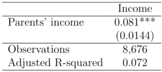
I start by showing estimates of intergenerational mobility using the standard specification, that is, the log-log income specification outlined in equation (1). β1 estimates whether par- ents’ place in the economic distribution matters for their child’s economic outcome. In a high mobility economyβ1 will be closer to zero, whereas in a low mobility economyβ1 will be closer to one. Estimates of intergenerational mobility in income are shown in Table 1, where I regress the log of child’s income on the log of parents’ income. All specifications control for age, gender, location (urban vs. rural), religion, and ethnicity. I do not find any gender difference in income mobility. The IGE estimate is 0.08 and significant at the 1 percent level. This low IGE coefficient indicates higher intergenerational mobility in Indonesia when estimated using income.5.
The intergenerational elasticity estimates can vary over the life of an individual. Children with high lifetime income have a steeper earnings profile when they are young, so the mobility estimates (IGE and rank-rank slope) are sensitive to the age at which we measure the child’s income. These estimates, however, stabilize around age 30 as compared to estimates at a
5United States is among the least mobile developed nations and most estimates of intergenerational elasticity fall between 0.3 and 0.5 (Chetty, Hendren, Kline, Saez, & Turner, 2014)
Table 1: Intergenerational Elasticity in Income Income
Parents’ income 0.081***
(0.0144)
Observations 8,676
Adjusted R-squared 0.072
Notes: Robust standard errors, in parentheses, are clustered at the dis- trict and year of birth level. All re- gressions include individual age and demographic controls. *** p<0.01,
** p<0.05, * p<0.1
lower age, which understates intergenerational persistence in lifetime income (Grawe, 2006;
Haider & Solon, 2006; Solon, 1999). To address this life-cycle bias in the mobility estimates, I include polynomial age controls (Corak & Heisz, 1999) in my regression estimates, as well as restricting the age of my sample for children to age 30 and above.
4.1.2 Intergenerational Rank Association
To estimate the rank correlation measure, I regress the child’s percentile rank in their gener- ation’s earnings distribution on their parents’ percentile rank in their generation’s earnings distribution (Dahl & DeLeire, 2008). OLS estimates of equation (3) give the estimate of intergenerational rank association (IRA). The results are presented in Table 2. The baseline estimate gives an IRA of 0.13. Similar to the IGE estimation, I include age controls (to account for life-cycle bias) and gender controls (to estimate gender difference in mobility) to estimate rank mobility.
Table 2: Intergenerational Rank Association
Percentiles Income
Parents’ income 0.132***
(0.0135)
Observations 8,676
Adjusted R-squared 0.166
Notes: Robust standard errors, in parentheses, are clustered at the dis- trict and year of birth level. All re- gressions include individual age and demographic controls. *** p<0.01,
** p<0.05, * p<0.1
All estimates are positive and significant at a 1 percent significance level. Similar to what I found with intergenerational mobility in income, this rank estimate shows lower income
mobility in Indonesia. For comparison, IRA estimates for the U.S., Canada, and Denmark are 0.34, 0.18, and 0.17, respectively (Chetty, Hendren, Kline, & Saez, 2014). This smaller rank slope, as compared to the U.S for example, suggests a lower gain in Indonesian chil- dren’s mean income rank as compared to children in these three countries, which suggests lower income mobility in Indonesia.
4.1.3 Absolute Mobility
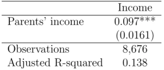
To ensure that the value of β1 is not driven by the change in standard deviations of parental and child income, I use equation (2) to estimate intergenerational mobility. The value of ρ is not affected by the changes in standard deviations or the possible evolution of the income distribution. The estimates ofρ are shown in Table 3. Intergenerational elasticity of income slightly increases to 0.097 from 0.080, with the lowerβ1 suggesting higher variance in income in parents’ income distribution.
Table 3: Intergenerational Elasticity: Rho Estimates Income
Parents’ income 0.097***
(0.0161)
Observations 8,676
Adjusted R-squared 0.138
Notes: Robust standard errors, in parentheses, are clustered at the dis- trict and year of birth level. All re- gressions include individual age and demographic controls. *** p<0.01,
** p<0.05, * p<0.1
By controlling for changes in variances and the differences in income in both generations, the results show lower intergenerational mobility in income in absolute terms, as compared to what I estimated for relative mobility.
4.1.4 Spline Estimates
I use the spline specification of equation (4) to estimate absolute intergenerational mobility.
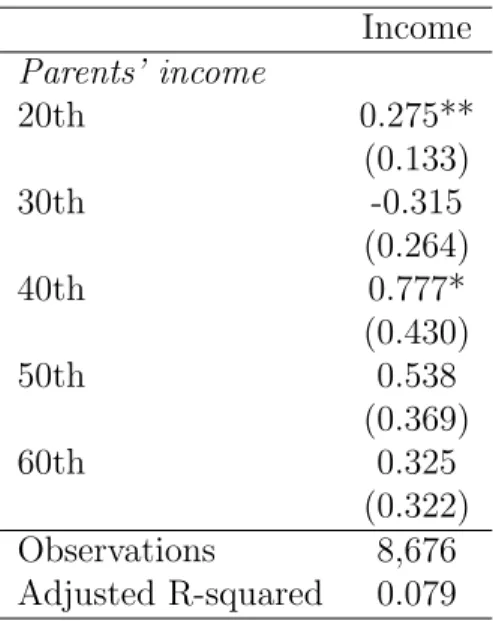
This specification allows the intergenerational estimates to vary along different points of the parental income distribution. Table 4 presents the estimates of spline regressions using income as a measure of economic mobility. Knots are set at 20th, 30th, 50th, and 60th percentile. I use percentiles of parent’s income, at the specified knots, and regress them on the child’s income, the estimation includes standard controls as discussed earlier.
I use the spline specification of equation (4) to estimate absolute intergenerational mobil- ity. This specification allows the intergenerational estimates to vary along different points of
Table 4: Absolute Mobility: Spline Estimates Income
Parents’ income
20th 0.275**
(0.133)
30th -0.315
(0.264)
40th 0.777*
(0.430)
50th 0.538
(0.369)
60th 0.325
(0.322)
Observations 8,676
Adjusted R-squared 0.079
Notes: Robust standard errors, in parentheses, are clustered at the district and year of birth level. All regressions include individual age and demographic controls. ***
p<0.01, ** p<0.05, * p<0.1
the parental income distribution. Table 4 presents the estimates of spline regressions using income as a measure of economic mobility. Knots are set at the 20th, 30th, 50th, and 60th percentiles. I use percentiles of parents’ income, at the specified knots, and regress them on the child’s income. The estimation includes standard controls as discussed earlier.
Overall, I found higher intergenerational mobility in income, as shown by the coefficient of 0.08. However, when we look at the breakdown at different percentiles of parents’ income, we find relatively lower income mobility. Higher elasticity estimates at the 20th, 40th, 50th, and 60th percentiles indicate lower income mobility. Income mobility is especially lower at the 40th percentile where the elasticity coefficient of 0.77 is very high. I also find absolute downward mobility at the 30th percentile, but the results are not significant. These results are in line with the intergenerational mobility estimates found for other countries such as the U.S., Canada, and Sweden.6
6Corak et al. (2014) report largest downward mobility from the top of the income distribution in Canada, followed by Sweden and least downward mobility in the United States. They find no difference in the upward mobility estimates for the bottom of the income distribution in these three countries. In Sweden, top 10 percent of the distribution has intergenerational elasticity of 0.9 (Hilger, 2015), (Chetty, Hendren, Kline, Saez, & Turner, 2014), and (Bj¨orklund et al., 2012).
4.2 Instrumental Variable Estimates
Following the methodology from section 3, the instrumental variable estimates are presented in Tables 5–8. For annual household income, the first stage results are shown in Table 5.
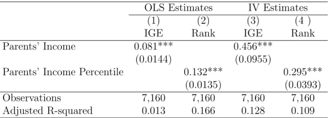
The instrument, 1993 parental income, is significant at the 1 percent level. The F-statistic for joint significance is also significant at the 1 percent level and is greater than 10. This shows that 1993 parental income is a strong instrument. To make the IV estimates compa- rable to OLS estimates, I first estimate relative mobility using parental income from 1997 in the RHS. The relative mobility estimate, using the OLS specification, gives an IGE of 0.14, which is higher than the IGE estimates using the 1993 parental income. The IGE coefficient estimated through an instrumental variable increases to 0.456 (see Table 6). This result is not surprising because the OLS estimate is biased downwards because of the measurement error.
This IV estimation shows the extent of the attenuation bias, which is large as the estimate increases from 0.08 to 0.465, and it also indicates how estimates of intergenerational mobility may overestimate mobility if the measurement error is not addressed properly (Ward, 2021).
This result indicates substantially lower intergenerational mobility in Indonesia, once the estimates are corrected for measurement error.
Table 5: Instrumental Variable: First Stage
1997 Income 1997 Income Percentile
1993 Income 0.1649***
(0.0095)
1993 Income Percentile 0.4094***
(0.0179)
Observations 7,160 7,160
Adjusted R-squared 0.148 0.209
F-statistic 298.952 522.843
Notes: Robust standard errors, in parentheses, are clustered at the district and year of birth level. All regressions include individual age and demo- graphic controls. *** p<0.01, ** p<0.05, * p<0.1
I also estimate intergenerational rank association using the instrumental variable method.
The relative mobility estimate (IRA) increases from 0.13 to 0.29 after correcting for mea- surement error. This coefficient suggests that, on average, a 10 percentile difference in rank in the parents’ distribution is associated with an expected 2.9 percentile difference in the child’s distribution. Both sets of results for IGE and rank estimation using instrumental variable are presented in Table 6, and their first stage results are shown in Table 5. Both sets of results indicate (1) the presence of random measurement error and attenuation bias and (2) lower intergenerational mobility in income in Indonesia.
I also use a Hausman test (Hausman, 1978) to show that the IV estimates are preferred.
I am able to reject the null of no measurement error in income. Therefore, the preferred set of results are the IV estimates. These results in themselves, and also when compared to mo-
Table 6: Instrumental Variable Estimates of Intergenerational Mobility OLS Estimates IV Estimates
(1) (2) (3) (4 )
IGE Rank IGE Rank
Parents’ Income 0.081*** 0.456***
(0.0144) (0.0955)
Parents’ Income Percentile 0.132*** 0.295***
(0.0135) (0.0393)
Observations 7,160 7,160 7,160 7,160
Adjusted R-squared 0.013 0.166 0.128 0.109
Notes: Robust standard errors, in parentheses, are clustered at the district and year of birth level. All regressions include individual age and demographic controls. ***
p<0.01, ** p<0.05, * p<0.1
bility estimates from other countries, suggest comparable or lower intergenerational mobility in income in Indonesia. For example, intergenerational elasticity in the U.S. is between 0.3 and 0.5 (Chetty, Hendren, Kline, & Saez, 2014). Wealth mobility in Bangladesh, another developing country, ranges from 0.53 to 0.77 (Asadullah, 2012). These numbers indicate the presence of lower intergenerational mobility in Indonesia relative to most developed coun- tries, as well as some developing countries.
4.3 Intergenerational Mobility in Consumption Expenditure
To my knowledge, the literature on intergenerational mobility only uses sources of current income to estimate intergenerational mobility. This data is normally collected at a certain point in life and as a result is susceptible to life-cycle bias. Intergenerational mobility could be estimated more accurately if researchers were able to measure income at around age 40 for both the parent and the child, which is the closest proxy to permanent income, or by using some other measure of permanent or lifetime income. To address this problem, I estimate absolute and relative mobility coefficients using both children’s and parents’ household per capita consumption expenditures, instead of income.
Consumption is a better measure of (economic) well-being in developing countries, espe- cially when the primary source of income is from agriculture or the informal sector. This gives us a better measure of commodity consumption by the household, such as food, clothing, and housing (Ravallion, 2015). Consumption is also a better proxy for lifetime income and is less susceptible to measurement error, as it is more easily recalled and measured (Aguiar
& Hurst, 2005; Hall, 1978; Stephens Jr, 2001). In most of the recent mobility literature, in- come comes from tax data or other federal income sources. In IFLS, households report their income, but because this income is not verified using any tax data or employment records, it can be misreported.7 In summary, in household surveys consumption is reported with less noise as compared to income, and therefore can be used to estimate intergenerational
7Tax compliance is low in Indonesia, with only 27 million out of an adult population of 185 million were
mobility.
In Indonesia, 72 percent of the population is employed in the non-agriculture informal sector (ILO, 2009). For these people, the best measure of household income is to use con- sumption expenditures because income sources are not always clear or correctly reported.
For example, self-employment and farm income is the primary income of many households, especially in rural areas (Deaton & Zaidi, 2002). If the primary source of income is not clearly defined or is dependent on seasonal agricultural outcomes, then income is also not a stable measure of the household’s economic well-being. Consumption, on the other hand, is less variable and more stable than income, particularly in agriculture economies such as Indonesia where rice production (farm income) is a main source of household income and consumption. We also cannot ignore the role of informal borrowing in developing countries:
households rely on informal sources (such as friends and family) to borrow money to smooth out their consumption. This effect is picked up in the consumption expenditure variable but not in income and savings.
In measuring consumption expenditures, recall that I separate household expenditures into food and non-food components. Non-food components include household expenditures on utilities, entertainment, education, and housing. Since non-food consumption is more affected by changes in income than food consumption is, this approach can provide a clearer sense of intergenerational mobility in Indonesia.
Relative mobility estimates (both IGE and IRA) are higher when estimated using con- sumption expenditures. Table 7 shows the results of intergenerational elasticity estimates and Table 8 shows the results of intergenerational rank association. The IGE coefficient is 0.26 using consumption expenditures, which indicates lower intergenerational mobility in Indonesia. When compared to uncorrected income estimates, this coefficient increased from 0.08 to 0.26. Estimates using total consumption and non-food consumption are very similar (0.255 versus 0.263), whereas IGE estimates using income are much lower.
Table 7: Intergenerational Elasticity in Consumption Expenditure
Consumption Expenditure Non-food Expenditure Parents’ total consumption expenditure 0.255***
(0.0200)
Parents’ non-food expenditure 0.263***
(0.0204)
Observations 12,640 12,640
Adjusted R-squared 0.102 0.121
Notes: Robust standard errors, in parentheses, are clustered at the district and year of birth level. All regres- sions include individual age and demographic controls. *** p<0.01, ** p<0.05, * p<0.1
registered as taxpayers in 2015. Ministry of Economic Affairs Indonesia also estimates that between 55 and 65 percent of employment is in informal sector, which is concentrated in rural areas.
The intergenerational rank association (IRA) measure also increases to 0.31 when es- timated using expenditures (from 0.08 when using uncorrected income). This result also indicates lower intergenerational mobility and the increase in IRA estimates further proves the presence of life-cycle bias and measurement error bias in previous estimates using uncor- rected income.
Table 8: Intergenerational Rank Association: Consumption Expenditure
Percentiles Consumption Expenditure Non-food Expenditure
Parents’ total consumption expenditure 0.317**
(0.0182)
Parents’ non-food expenditure 0.321***
(0.0195)
Observations 12,640 12,640
Adjusted R-squared 0.111 0.122
Notes: Robust standard errors, in parentheses, are clustered at the district and year of birth level. All regres- sions include individual age and demographic controls. *** p<0.01, ** p<0.05, * p<0.1
As noted earlier, I estimate mobility using non-food household expenditures as well. An increase in household income is mostly reflected in an increase in non-food consumption such as education, utilities, etc.8 Table 7 column 2 and Table 8 column 2 show the results using non-food per capita consumption expenditures. The results are similar to IGE and IRA estimates using total expenditures: the IGE estimate is 0.26 and the IRA estimate is 0.31.
These results again point to the presence of life-cycle and measurement error bias. They also indicate lower intergenerational mobility. These elasticity estimates indicate lower relative mobility in Indonesia when compared to the U.S., Sweden, and Canada (Corak et al., 2014).
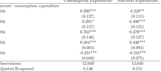
Spline estimates are also in line with my findings of lower intergenerational mobility when estimated using consumption expenditures. As we can see in Table 9, there is lower intergenerational mobility at the bottom 20th, 30th, and 40th percentiles of the consumption distribution, for both total consumption expenditures and non-food expenditures. Compared to the overall distribution, where the elasticity coefficient is 0.31, we see that families at the bottom of the consumption expenditure distribution experience even lower intergenerational mobility, as can be seen by the coefficients of 0.39, 0.29, and 0.76 at the 20th, 30th, and 40th percentiles, respectively. This distributional breakdown of intergenerational mobility sheds more light on the mobility scenario in Indonesia and highlights how people at the bottom of the income and consumption distribution are at a higher disadvantage, compared to people at the top of the distribution.
In comparison to the income and IV estimates of intergenerational elasticity, consumption seems to be the preferred measure of households’ economic well-being and economic mobility.
Consumption not only gives us a better measure of households’ permanent income, which we are not able to observe directly from the data, but it also does not suffer from measurement
8Aguiar and Hurst (2005) and Stephens Jr (2001)
Table 9: Absolute Mobility: Spline Estimates
Consumption Expenditure Non-food Expenditure Parents’ consumption expenditure
20th 0.393*** 0.228**
(0.127) (0.115)
30th 0.291* 0.406***
(0.157) (0.125)
40th 0.763*** 0.479***
(0.146) (0.127)
50th 0.284*** 0.430***
(0.085) (0.084)
60th -0.231*** -0.310***
(0.048) (0.075)
Observations 12,640 12,640
Adjusted R-squared 0.136 0.151
Notes: Robust standard errors, in parentheses, are clustered at the district and year of birth level. All regressions include individual age and demographic controls. *** p<0.01, ** p<0.05, * p<0.1
error to the extent income does. This is clearly observed when the IV estimates increase in magnitude. Between IV and the consumption expenditure estimates, I again argue that consumption is the preferred measure because with the instrumental variable we are only able to estimate the local average treatment effect instead of the average treatment effect (Angrist & Krueger, 2001). In this case, the local average treatment effect is only for those parent–child pairs for whom we have parental income in both 1993 and 1997, whereas for consumption expenditures the sample includes a large number of households, as well as those members of the household who are part of the labor market but did not report their income.
Therefore, the elasticity estimated using consumption expenditures is far more accurate and gives a more reliable measure of intergenerational elasticity in Indonesia.
5 Robustness
In this section, I show that the estimates of intergenerational mobility are robust to different specifications. Here I will also attempt to show the internal and external validity of my estimates of intergenerational mobility.
5.1 Attrition
Attrition and tracking are major problems in survey data. If attrition in the survey is not random then it could present some bias in the estimates. I check for attrition in my sample for parents whose children were present in the 1993 survey but who dropped out of the 2014 survey. My primary goal is to check whether I have selective attrition by parental income.
If attrition is selective by parental income, then the mobility estimates will be biased. To check for attrition, I follow Hanaoka et al. (2018) and McKenzie (2015).
First, I test the null hypothesis that the mean income and mean years of schooling of parents whose children attrited (N=1,508) and those who did not is the same. I could not reject the null hypothesis for mean income (p-value= 0.982) and for mean years of schooling (p-value= 0.437). This implies that the mean income and years of schooling of parents whose children attrited is not statistically different from the non-attriters.
Furthermore, I regress the dummy variable for attrition on parental income, years of schooling, and per capita household consumption expenditures, to check if attrition is corre- lated with any of these variables. The results are shown in appendix Table A.4. The results from Table A.4 show that attrition is not correlated with parental income and parents’ years of schooling. These two sets of results show that attrition is not selective by parental income or parents’ years of schooling, suggesting that the estimates of intergenerational mobility in income are unbiased.
I repeat the same procedure to check if attrition is correlated with per capita household consumption expenditures. The t-test shows that the null hypothesis of zero mean difference in per capita household consumption expenditures should be rejected (p-value= 0.00). The regression results from Table A.4 show that attrition is correlated with per capita household consumption expenditures. Hence, attrition is selective in this case.
To correct this, I use inverse probability weights (IPW). The attrition-adjusted estimates of intergenerational elasticity for consumption expenditures are shown in appendix Table A.5. The IGE estimates are slightly larger than the estimates from the entire sample (0.255 for the entire sample and 0.305 after adjusting for attrition). This indicates slightly lower intergenerational mobility (in consumption) in Indonesia, once the data is adjusted for at- trition.
5.2 Co-residence
In this section, I estimate mobility for a sample of children who live in multi-generation households. This includes the children’s sample from 2014 whose parents are still living with them in the same household. My sample has approximately 3000 children who live in co-resident households, and out of them I have complete household information on 1,222 individuals. Family linkages are especially important in developing countries, where families rely on informal forms of borrowing to smooth consumption and to invest in human capital (Cameron & Cobb-Clark, 2008; Raut & Tran, 2005). Therefore, pooled household income and family networks play an important role in determining social mobility. LaFave and Thomas (2017) suggests that family linkages are critical in Indonesia, where families not only support each other in times of a negative shock but also invest in the next generation.
The co-residence estimates are shown in appendix Table A.6. The elasticity coefficients
for income and consumption are all lower than the estimates for the entire sample given in Table 1 and Table 7. These lower estimates suggest relatively higher mobility for children who live in co-resident households. For example, the IGE estimate using consumption ex- penditures is 0.25 for the entire sample but 0.18 for the co-resident household sample. These estimates suggest that households do pool resources, and that this helps them achieve higher intergenerational mobility.
Table A.6 also shows the measurement error-corrected estimates (using the IV method) for the co-resident households. These estimates don’t change when compared to the IV estimate for the entire sample, reaching 0.45 in both cases. Estimates from the preferred method using consumption expenditures capture the co-resident impact more accurately as households pool resources, and they show higher economic mobility for households in In- donesia.
5.3 Nonparametric Analysis
Instead of assuming a linear relationship between parents’ income and children’s income, I use non-parametric estimation for intergenerational elasticity. Non-parametric regression yields consistent estimates of the mean function which are robust to functional form mis- specification.9
The results from the non-parametric estimation are reported in appendix Table A.7.
Overall, these results are closer to the linear estimation, suggesting the estimates of inter- generational mobility are not sensitive to the functional form. The marginal effect of parental income on children’s income is 0.08 and significant; this estimate is closer to the linear re- gression estimate. Similarly, the marginal effect of parental consumption expenditures on children’s consumption expenditure is 0.32 and significant. This is slightly larger than the OLS estimate. Lastly, the marginal impact of parental non-food consumption expenditures on children’s non-food consumption expenditures is 0.28.
5.4 Restricted Sample for Consumption Expenditure
In order to better understand intergenerational mobility estimates using consumption ex- penditures, and also to form a better comparison with income-based estimates, I restrict my sample to individuals for whom I have information on both income and consumption expen- ditures. I estimate both rank mobility and elasticity estimates for this restricted sample for consumption expenditures. These results are shown in Table A.8.
Comparing these results to the full sample (shown in Tables 7 and 8), the mobility estimates do not change substantially. For the intergenerational elasticity estimate, the
9I use Kernel regressions as a non-parametric technique to estimate the marginal effect.
coefficient changes from 0.26 to 0.22. Both of these estimates are larger than the OLS es- timates of income, suggesting relatively lower intergenerational mobility. Similarly, for the rank estimate, the coefficient changes from 0.31 to 0.24. Both of these estimates are larger in magnitude than the uncorrected OLS estimates using income, which suffers from mea- surement error bias. This estimate shows that a 1 percentage point increase in parental rank leads to a 0.244 percentage point increase in children’s rank, as estimated using consumption expenditures. These estimates are not sensitive to the sample size and suggest that estimates of intergenerational mobility using income suffer from attenuation bias.
5.5 Sample Representation
The original IFLS sample in 1993 surveyed 13 out of 26 provinces in Indonesia. Although more households were added to the sample in following waves, it still does not fully rep- resent the entire Indonesian population. To show how representative my sample is of the Indonesian population, I use data from the census survey, SUPAS. The intercensal survey is conducted every ten years by the Central Bureau of Statistics of Indonesia. I use the 2010 survey. Since the income variable is not well-reported in SUPAS, I use years of schooling to check the external validity of my sample. Education itself is also a good indicator of earnings and economic outcomes.
The kernel density graph of years of schooling from both the IFLS and SUPAS is shown in Figure A.5. Both distributions are bimodal, which shows that most people in Indonesia complete 6 to 12 years of schooling. The mean and the standard deviation of both distribu- tions are similar, which suggests that IFLS does in fact represent the Indonesian population.
6 Conclusion
I use data from multiple waves of the Indonesian Family Life Survey to show that intergener- ational mobility estimates are sensitive to measurement error bias and life-cycle bias. Once I control for individual characteristics, random measurement error, and life-cycle bias, I find low intergenerational mobility in Indonesia. Indonesia is the fourth most populous country in the world, and it is facing concerns of rising inequality.10 This underscores the impor- tance of studying intergenerational mobility for Indonesia and the need for policy reforms in areas which will improve the economic mobility of the country’s large and growing youth population.
Since we are unable to observe permanent income from the IFLS data, consumption ex- penditures can be used a better measure of lifetime income because it takes into account the life-cycle bias and co-residence in developing countries. When I use consumption expendi- tures to measure intergenerational mobility, the IGE estimate increases substantially from
10Gini coefficient of 0.4 and 40th rank in countries with largest inequality according to the recent World Bank report.
0.08 to 0.25, showing that this may be an important factor for precisely measuring intergen- erational mobility in developing countries. I also analyze both relative and absolute mobility.
These results, along with the intergenerational rank association of 0.57 and spline estimates of absolute mobility, indicate a low degree of absolute and relative intergenerational mobility in Indonesia. This is comparable to the intergenerational elasticity estimate in Bangladesh, which is between 0.5 and 0.77 (Asadullah, 2012).
I argue that consumption expenditures data can be used as a measure of households’ eco- nomic status to estimate intergenerational mobility. This has more significance in developing countries where the unavailability of income and tax data present a concern. Furthermore, consumption expenditures are a superior measure of households’ economic status in devel- oping countries, especially compared to income and education. Household-based economic activities and dependence on informal sector employment means income data does not ac- curately reflect the economic status of a household, whereas consumption takes into account all unreported sources of income. Households in developing countries also rely on informal borrowing and pooling of household resources in co-resident households, which enables them to smooth their consumption.
Estimating intergenerational mobility using income data may underestimate mobility if households have access to informal sources of funding. This also undermines the role played by welfare programs, which aim to provide liquidity to households to maintain their con- sumption expenditures. We cannot ignore the role of extended family in providing economic assistance in hard times, especially in a country like Indonesia that is vulnerable to several natural disasters. Findings from this paper show that co-residence households experience higher intergenerational mobility, this might indicate that economic support from family members will minimize their risk in times of an economic shock or a natural disaster. Lastly, we should encourage countries to gather data on consumption expenditures and build on our existing databases on consumption expenditures, such as the Living Standard Measurement Study (LSMS), to gather more evidence on intergenerational mobility in developing countries.
This paper contributes to the existing literature on intergenerational mobility and more specifically, to the still emergent literature on developing countries. Most of this literature uses education data, but education is not a very precise measure of the economic status of a household—especially since the returns of education vary widely by gender, caste, and socio-economic status of the household. Little research has been done on intergenerational mobility, especially income and consumption mobility, in developing countries,11 and, to my knowledge, no studies have been done on Indonesia.
This evidence from Indonesia, combined with intergenerational mobility estimates from the U.S. (Chetty, Grusky, et al., 2017), Bangladesh (Asadullah, 2012), India (Azam, 2016), Philippines (Bevis & Barrett, 2015), and Sweden (Corak et al., 2014), highlights global in- cidence of lower both absolute and relative intergenerational mobility. This paper paves the way for using a better measure of households’ economic well-being to estimate inter-
11Bevis and Villa (2017), Bevis and Barrett (2015), Asadullah (2012), and Asher et al. (2017)
generational mobility, ideally using consumption expenditures given that accessing reliable consumption data in developing countries is far easier than accessing reliable income data.
The main contribution of this research is that intergenerational elasticity estimates us- ing income suffer from measurement error and the size of the bias could be very large. In contrast, consumption expenditures are a better measure of intergenerational mobility, es- pecially in developing countries where administrative data, tracking both parents and their children over a long period of time, are lacking. I also find that by pooling resources (co- residence households), households are able to experience higher economic mobility. This calls attention to the need for designing policies that boost consumption, and to understand family dynamics and pooling of resources in more detail.
Table A.1: Summary Statistics Income
Children with parents in these quantiles
Child’s Variables 0-25 25-50 50-75 >75
Income (USD) Mean 1,117 1,314 2,037 1,642
(s.d) (3,285) (5,232) (1,577) (9,856)
Age Mean 31.16 30.01 30.26 28.20
(s.d) (8.35) (8.18) (7.82) (8.94)
Years of Schooling Mean 8.59 9.53 11.27 11.18
(s.d) (4.13) (3.84) (3.50) (3.52)
Observations 1,321 2,222 2,349 5,899
Consumption Expenditure
Consumption Expenditure (USD) Mean 460 723 920 854
(s.d) (525) (788) (1,183) (850)
Age Mean 27.42 31.77 33.16 32.14
(s.d) (8.99) (7.06) (7.23) (8.10)
Years of Schooling Mean 9.84 11.25 12.85 11.98
(s.d) (3.72) (3.70) (3.12) (3.52)
Observations 5,449 5,375 2,472 68
Controls
Urban Percentage 62
Male Percentage 51
Muslim Percentage 89
Javanese Percentage 24
Household Size Percentage 4
Notes: Poverty line in Indonesia is USD 24.8 monthly (USE 297.6 annual) according to the BPS, 2016.
Table A.2: Real Household Income Income
Children Parent 1993 Parent 1997
Mean 1,584 178 924
Standard Deviation (10,560) (2,442) (1,584) Quantiles
<25 34.99 0.12 82.48
25-50 383.84 0.48 335.23
50-75 976.80 1.29 772.20
>75 5,101.80 706.20 2,514.60
Observations 11,791 14,064 23,111
Notes: All values annual and in USD. Poverty line in Indonesia is USD 24.8 monthly (USD 297.6 annual) (Source: BPS, 2016).
26