Sejarah dan Perkembangan Superkonduktor ke 3 - Spada UNS

FISIKA

SUPERKONDUKTOR

oleh :

Fuad Anwar

LANJUTAN

SEJARAH DAN PERKEMBANGAN

S U P E R K O N D U K T O R

PENGERTIAN SUPERKONDUKTOR :

MUNCUL FENOMENA

SUPERKONDUKTIVITAS :

•  = 0

• Efek Meissner

• dsb.

JIKA

T < T

_c

H < H

_c

DAN

SEJARAH PENEMUAN SUPERKONDUKTOR :

 Tahun 1908 : Heike Kamerlingh Onnes dan Timnya (Leiden University) berhasil mencairkan Helium (suhu sekitar 1 K)

 Tahun 1911 : Heike Kamerlingh Onnes dan Timnya

melakukan pengukuran hambatan merkuri sebagai fungsi suhu R(T).

Hasilnya :

 R=0 pada T=4,2 K

 Merkuri : jenis superkonduktor

 Merkuri mempunyai suhu kritis

Tc =4,2 K

Heike Kamerlingh Onnes “the gentleman of absolute zero”, discovered Superconductivity on April 1911. Onnes won the Nobel Prize in 1913, just two years after his incredible discovery. Onnes died in 1926.

In 1898 Onnes’ rival, James Dewar, beat him in the race to liquefy hydrogen.

Onnes then moved on to a new goal, liquefying helium, and this time, Onnes beat Dewar in the race, producing the first liquid helium in July 1908.

Though he only liquefied a tiny amount of helium at that time, the liquefaction of helium made it possible to cool other substances to such low temperatures.

Onnes managed to cool the liquid to about one degree above absolute zero, at the time the coldest temperature ever achieved.

“The resistance of pure mercury at helium temperatures,” Communications from the Physical Laboratory at Leiden, April 1911.

“On the Sudden Change in the Rate at which Resistance of Mercury Disappears.” November 1911. Soon after finding the effect in mercury, Onnes showed that tin and lead also become superconducting at low temperatures.

In 1913 Onnes first used the term “supraconductivity,” to describe the effect;

later he changed it to “superconductivity.” By 1914 he had found another interesting feature: he started a supercurrent flowing in a lead wire, and a year later, found that it was still flowing, with no noticeable change. Onnes himself had believed that quantum mechanics would explain the effect, but he wasn’t able to produce a theory.

Heike Kamerlingh Onnes dan Timnya juga menemukan :

 Beberapa unsur lain juga menunjukkan sifat superkonduktif dengan harga Tc yang berbeda.

 Sifat superkonduktif akan hilang jika superkonduktor dikenai

medan magnet melebihi harga tertentu (disebut medan kritis Hc)

Superkonduktor unsur jenis lain :

Penemuan superkonduktor suhu tinggi

Muller dan Bednorz, 1987

Paul Chu, 1988

Penemuan superkonduktor suhu tinggi

Jenis Superkonduktor

No Jenis bahan T

_c

( K )

1. Unsur : Al

Nb 1,2

9,2 2. Paduan logam/senyawa biner :

Nb-Ti

MgB2 9

39 3. Superkonduktor heavy fermion :

UBe

₁₃

UPd

₂

Al

₃

0,85 2 4. Superkonduktor organik :

β

_L

-(BEDT-TTF)

₂

I

₃

-(BEDT-TTF)

₂

Cu(NCS)

₂

1,5 10,4 5. Superkonduktor oksida :

La

_2-x

Sr

_x

CuO

₄

YBa

₂

Cu

₃

O

_7-x

38 92 6. Superkonduktor pnictide :

LiFeAs

GdFeAsO

_1-x

18

53,5

PERTEMUAN KE 3

LANJUTAN

SEJARAH DAN PERKEMBANGAN

S U P E R K O N D U K T O R

SIFAT MAGNET SUPERKONDUKTOR

Walter Meissner

GAMBARAN SIFAT SUPERKONDUKTOR :

lihat video 1-2

JENIS SUPERKONDUKTOR :

Superkonduktor

Superkonduktor Tipe I

Superkonduktor Tipe II

H

_c

H

_c1

H

_c2

(pada superkonduktor bongkahan/bulk)

SUPERKONDUKTOR BONGKAHAN ( BULK )

Ada 2 tipe superkonduktor :

• superkonduktor tipe I

• superkonduktor tipe II

Superkonduktor tipe I Superkonduktor tipe II B=0

-M

H

_ekt

-M

B0

keadaan campuran B=0

keadaan Efek Meissner

H

_ekt

H

_c2

H

_c1

H

_c

H

_c

keadaan

Efek

Meissner

SUPERKONDUKTOR TIPE II

(memperhatikan batas permukaan)

H ext

H

_c1

H

_c2

H

_c3

superkonduktivitas sempurna

superkonduktivitas sebagian

(mixed state)

superkonduktivitas permukaan

normal

fluks magnet dapat menerobos superkonduktor secara parsial fluks magnet terkuantisasi dalam bentuk vorteks

1 vorteks :

e e

h  

  

0

2

APLIKASI SUPERKONDUKTOR :

 penghantar arus listrik tanpa kehilangan energi

 pembangkit medan magnet super tinggi dalam MRI

 penyusun kumparan levitasi magnet MAGLEV

 pengukur medan magnet sangat sensitif dalam SQUID

 dan sebagainya

Gambaran Aplikasi Superkonduktor

GAMBARAN APLIKASI SUPERKONDUKTOR

lihat video 3

Teori Superkonduktor :

• Teori fenomenologi superkonduktor :

Teori London dan Teori Ginzburg-Landau

• Teori mikroskopis : Teori BCS

Bardeen, Cooper, Schrieffer (BCS)

Lev D. Landau and V. Ginzburg

Penemu Teori Superkonduktor

A.A. Abrikosov

Gambaran Teori BCS

Superconducting Gap in the electronic spectrum – Order parameter.

GAMBARAN ELEKTRON SUPER

lihat video 4

TEORI GINZBURG-LANDAU

Memperkenalkan Rapat Energi Bebas Gibbs Superkonduktor : Memperkenalkan konsep parameter benahan (ψ) :

• menunjukkan keberadaan sifat superkonduktivitas

• |ψ(r)|

²

menyajikan rapat lokal elektron super

CATATAN :

 dan A bergantung pada ruang saja

   

2 0

0 2 2

4 2

2 1 2

2 1

,

H

ext

B A

A

 















 



 

   













s

s n s

i e m

T f

g

Keterangan :

g

_s

: rapat energi bebas Gibbs superkonduktor f

_n

: rapat energi bebas Gibbs keadaan normal ψ : parameter benahan

ћ : tetapan Planck dibagi 2π, μ

₀

: permeabilitas ruang hampa,

A : potensial vektor magnet di dalam superkonduktor B : induksi magnet di dalam superkonduktor

H

_ext

: intensitas medan magnet luar

e

_s

dan m

_s

: muatan dan massa elektron super

 (T) dan  : koefisien ekspansi rapat energi bebas Gibbs Catatan :

 = konstanta positif, bukan fungsi T

  0 1 , di mana   0 adalah pada 0 K

)

(   

 



 

 T

T T T

c









Minimisasi Rapat Energi Bebas Gibbs Superkonduktor terhadap ψ(r) dan A(r) menghasilkan :

Persamaan Ginzburg-Landau Pertama

Persamaan Ginzburg-Landau Kedua

J

_s

(r) : rapat arus super

            



 



    













r ie r

r r

r im r

e

r r

s s

s

A

A J

_s

2

2

2

) ( )

(









 



    ( ) 0

) 2 ( )

( )

(

2 2

2

 



 

   





 e r r

m i r

r r

T

^s

s











 A





PERSAMAAN SYARAT BATAS :

tanpa efek proksimitas

ada efek proksimitas

b : panjang ekstrapolasi

DARI TEORI GINZBURG-LANDAU, didefinisikan :

• panjang koherensi :

• panjang penetrasi London :

• parameter Ginzburg-Landau :

) ( ) 2

(

2

T T m

s



  

) ) (

(

₂

0

e T

T m

s s





  

2 2 0

2

2

) (

) (



s s

e m T

T







   

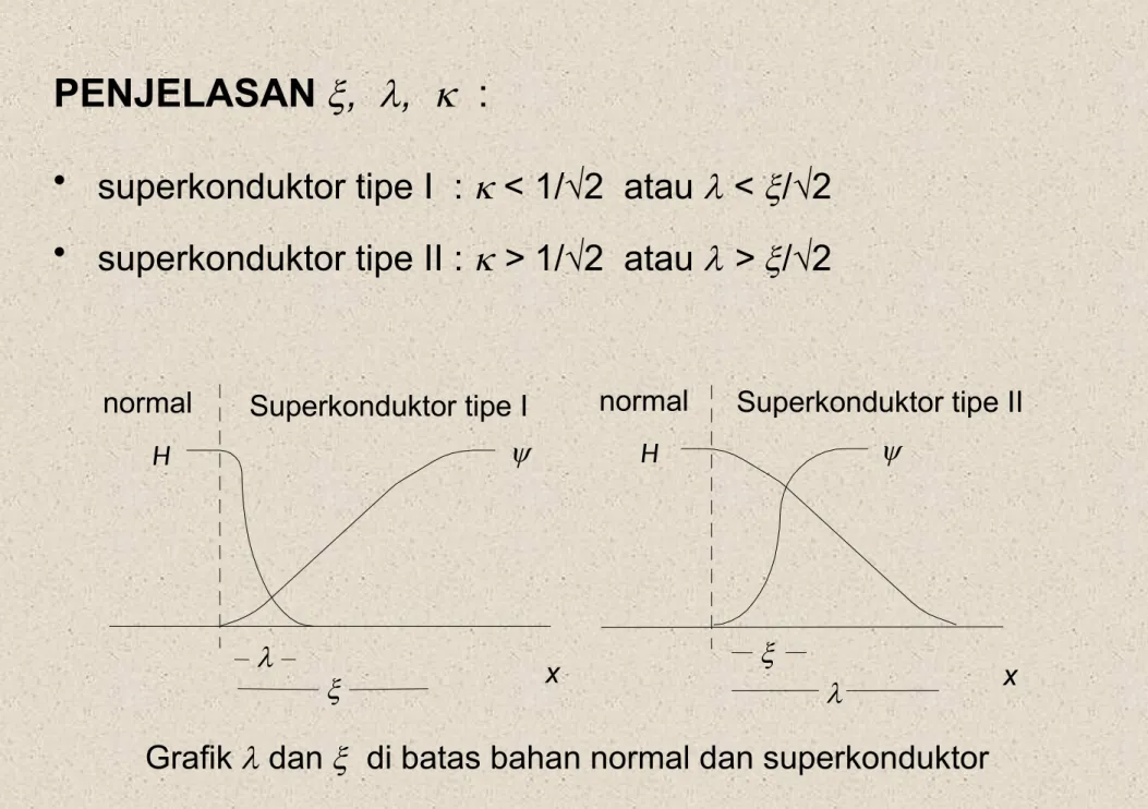
PENJELASAN  ,  ,  :

• superkonduktor tipe I :  < 1/√2 atau  <  /√2

• superkonduktor tipe II :  > 1/√2 atau  >  /√2

Grafik  dan  di batas bahan normal dan superkonduktor

H

x H

Superkonduktor tipe I

 



normal normal Superkonduktor tipe II





 x

DARI TEORI GINZBURG-LANDAU, diperoleh :

• Medan kritis rendah :

• Medan kritis tinggi :

• Hubungan antara Hc

₁

dan Hc

₂

:

• Medan kritis permukaan :

Hc

_3//

(T)=1,695 Hc

₂

(T) Hc

₃

 (T)=Hc

₂

(T)

di mana

H

_ext

sejajar permukaan superkonduktor H

_ext

tegak lurus permukaan superkonduktor

     

 

 



 ln 2 ln

2

₀ ²

1

s s

s

m

T e

T T e

Hc    

   

 

²

0 0 2

2

T e e

m T T

Hc

s s s



 

 

 



   

   

2 2 2

2

1

2

ln ln





 Hc T T

Hc T T Hc

Hc        

2

2 0

2

 



 T Hc T T

Hc  

GAMBARAN VORTEKS :

lihat video 3