superconductivity as a structural characterization tool

IN AMORPHOUS MATERIALS

Thesis by

Bruce Montgomery Clemens

In Partial Fulfillment of the Requirements for the Degree of

Doctor of Philosophy

California Institute of Technology Pasadena, California

1982

(Submitted September 22, 1982)

TO MY PARENTS

ACKNOWLEDGEMENTS

I would like to acknowledge the support and encouragement of my adviser, Professor William Johnson, whom I admire as a scientist and a person. I feel I was very lucky to have as an adviser a person who possesses a great deal of knowledge and a joy in sharing it with others. I would like to thank Professor Johnson for introducing me to the field of superconductivity and I would like to thank both Professor Johnson and Professor Pol Duwez for introducing me to the field of amorphous and metastable materials.

I would like to thank Dr. Michael Tenhover for his assistance and interest in this work. For technical assistance I would like to

acknowledge the friendly support of Concetto Geremia, Angela Bressan, Sumio Kotake, Jue Wysocki, Hiπ-Wiπg Kul, and the staff of the Bitter Magnet Lab. I would like to thank Robert Schulz for his help in resistivity measurements and computerization of the critical current apparatus. I am grateful to Madhav Mehra for a fruitful collaboration in the study of sputtered films and I wish to thank Dr, Marc-Aurele Nicol et, Bai Xien Liu and Roily Gaboraiud for their part in the collaborative study of ion beam mixed materials.

I would like to acknowledge Dr, Randall Feenstra, Reuben Collins, Stuart Hopkins, Dr. Konrad Samwer, Dr. Arthur Williams and Lowell Hazelton for helpful conversations,

I am grateful to Carolyn Meredith and Vere Snell for their cheerful and efficient typing of this manuscript.

Most of all I wish to thank Susan, my wife, for her faith and support. Those who know me realize that she was responsible for a turning point in my life and career as a scientist.

For financial support I acknowledge the Department of Energy and the International Business Machine Corporation.

ABSTRACT

This thesis presents the use of superconductivity as a structural probe for studying amorphous and metastable materials. The charac­

teristics of the superconducting state which facilitate its use as a probe are explained, followed by a description of some of the

properties of the materials studied. The superconducting measure­

ments performed were critical current, transition temperature and upper critical field. Materials prepared by rapid quench from the melt, sputter deposition and ion beam mixing were studied. The critical current measurements performed on liquid quenched materials reflect three pinning mechanisms. Crystalline inclusions in otherwise amorphous (Moθ θRuθ 4)30^1 ∙jq≡iq Produced a dramatic increase in critical current. The pinning in purely amorphous (Μοθ θRuθ 4)32^8 was shown to be affected by pinning by surface roughness on the sample edges, This contribution can be eliminated by a proper sample

geometry and electropolish treatment. The bulk pinning in purely amorphous (Moθ gRu0 4)g2βΙ8 was s*10wn t0 -first decrease and then increase as a function of annealing time. This reflects the dis­

appearance of quenched in inhomogeneous strains and excess volume defects followed by the growth of an inhomogeneity such as composi­

tional phase segregation during an anneal. The upper critical field was measured for liquid quenched (Moθ θRuθ 4)1_χΒχ for x = 0,12, 0,18 and 0.22 both before and after an anneal. The annealed samples exhibited greater transition widths and more curvature in the H (T)

curves than the unannealed samples which are evidence for a growth of inhomogeneities upon annealing. Measurements on sputter deposited (Moq gRuθ 4)g2β]8 were performed on samples sputtered in low (5 μn) and high (75 ‰m) Ar pressure, The material sputtered in low Ar pressure had a greater drop in Tc than the liquid quenched material and a pinning profile which exhibited a peak near H . The sample

c2

sputtered in high Ar pressure was very inhomogeneous as evidenced by transition width and flux pinning force profile. Measurements were performed on ion beam mixed MθggRu^g. The structure consisted of an amorphous matrix with crystalline inclusions. The pinning

profile was characteristic of a strong pinning mechanism, The pinning force decreased then increased as a function of ion beam dose. This reflects the destruction of the remnants of the original structure followed by the formation of an inhomogeneity such as σ-MoRu or Xe gas bubbles during ion beam irradiation.

TABLE OF CONTENTS

I. Introduction 1

A. Superconductivity as a Materials Structural 1 Probe

B. Historical Background 2

II, Theoretical Background 4

A. Superconductivity 4

1, Microscopic Theory of Superconductivity 4

a. General Theory 4

b. Applied to Amorphous Materials 7

2, Ginsburg-Landau Theory 8

a. General Theory 8

b. Applied to AmorphousMaterials 16

3, Flux Pinning 18

B, Amorphous Materials 32

1, Formation and Structure 32

2. Transformation from the Amorphous State 35

III. Experiment 39

A. Sample Preparation 39

1. Liquid Quench 39

a. Piston and An/il 39

b. Melt Spin 41

2. Sputter Deposition 44

3. Ion Beam Mix 45

Β, Superconducting Measurements 46

1. Transition Temperature 46

2. Upper Critical Field 47

3. Critical Current Density 51

IV. Measurements on Liquid Quenched Materials 57

A, Flux Pinning 57

1. Pinning by Crystalline Inclusions 57

2. Pinning by Surface Roughness 70

3. Bulk Pinning in Purely Amorphous Materials 81

B, Upper Critical Field 92

V. Measurements on Sputter Deposited and Ion Beam

Mixed Films 98

A, Sputter Deposition 98

B. Ion Beam Mixed Films 109

VI. Summary 116

References 120

LIST OF TABLES

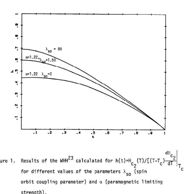
1. Pinning force field dependence for the various cases in the dynamic pinning model.

2. Specifications for superconducting Nb-Tl solenoid magnet.

3. Structure, superconducting transition temperature, and critical field gradient for (Moθ gRuθ 4qb^

∣

Q samP^es studied.

4. Composition, condition, small angle x-ray scattering, transition temperature, critical field gradient, and transition width for

(Mo06Ruθ4)1-χBχ samples.

5. Preparation condition, transition temperature, critical field gradients, and transition widths for samples of sputtered

(m°0.6ru0.4⅛2b18,

6. Xenon ion dose, transition temperature, critical field gradient, critical field at 4.2 K determined from resistive measurements

(4.2)) and flux pinning measurements

pinning force parameter for ion beam mixed Mo^^Ru^^ samples.

(H (4.2)), and flux Cn

LIST OF FIGURES

dHc.

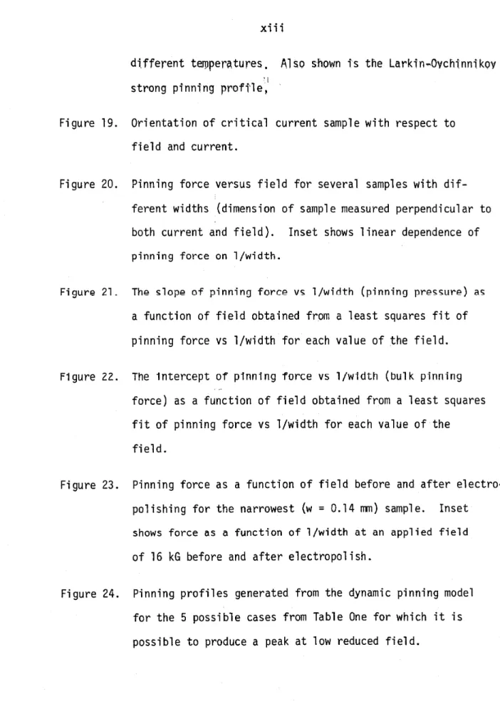
Figure I. Results of the WHH23 calculated for h(t)=H (T)∕[(T-T ) 2 ]

C£ c οι 1*

for different values of the parameters λsθ (spin c orbit coupling parameter)and a (paramagnetic limiting

strength).

Figure 2. Reduced field h(r) and order parameter ψ(r) as a function of position near an isolated vortex in a material where

λ∕ξ = 20.14.

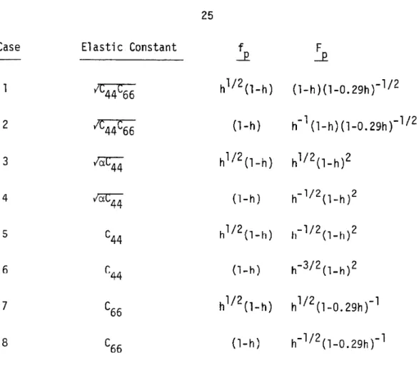
Figure 3. Pinning profiles for dynamic pinning model in non-diverging cases. Case numbers refer to Table 1.

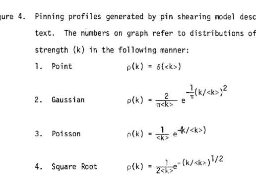
Figure 4. Pinning profiles generated by pin shearing model described in text. The numbers on graph refer to distributions of pin strength (k) in the following manner:

1. Point p(k) = δ(<k>)

2 Gaussian p(k)

2 ^-l(k∕<k>)2 π<k> c

3. Poisson P(k) _ 1 p4∕<k>)<k>

4. Square Root p(k) _ 1 n-(k∕<k>)lz2 2<k>c

Figure 5. Pinning profiles generated by Larkin-Ovchinnikov pinning

model for different values of the pinning strength parameter D.

Figure 6. Pinning profiles generated by Larkin-Ovchinnikov pinning model. Numbers on graph refer to distributions of pin

strength (k) in the following manner:

1. Point p(k) = s(<k>)

2. Gaussian „(

∖

j

∖

_ 2 k∕<k>)2 pk^ π<k> e " *

3. Poisson P(k)=⅛(^>

4. Square Root p(k) ⅛<kz<k>,v2

Figure 7. Radial distribution function for sputtered (Moθ gRuθ 4)g2B18·

Figure 8. Piston and anvil splat quenching technique.

Figure 9. Melt spinning apparatus.

Figure 10. Reduction in field as a function of position (x) along the axis of the solenoid measured from the center position.

Solid line is theoretically expected reduction.

Figure 11. Critical current probe end showing voltage and current contacts.

Figure 12. Typical I-V curves at different applied fields taken during a computerized critical current run. Points are data values and solid curves are second order polynomial fits. Also shown is a solid line at V = 0.5 μV, corresponding to a 1/2 μV criteria.

Figure 13. Results of structural analysis of amorphous

(m°O.6ruo.4⅛Osi1Ob1O with 0'1 -0.4% crystalline inclusions.

Shown are a) x-ray diffraction pattern, b) electron micro­

graph, c) electron diffraction pattern of a typical area.

Figure 14. Results of structural analysis of amorphous

^°0.6Ru0.4^80B^10B10 wι't*1 crystalline inclusions.

Shown are a) x-ray diffraction pattern, b) electron micrograph, c) electron diffraction pattern of a typical area.

Figure 15. Upper critical field H versus temperature for amorphous c2

and amorphous plus crystalline inclusions

(m°0.6ru0.4^80si'10b10* Also shown are linear extra­

polations to the data and curves from the Maki theory fit to the data.

Figure 16. Critical current as a function of applied field for

a) amorphous (Moθ gRuθ 4)go^hoBl'lO and b) amorphous plus crystalline inclusions (Moθ gRuθ 4)θθSi1θB1θ.

Figure 17. Pinning force as a function of field for amorphous (Moθ gRuθ 4)8O^-*iob1O* Also s*ι0wπ is the theoretical result of the dynamic pinning model.

Figure 18. Reduced pinning force as a function of field for amorphous plus crystalline inclusion (Moθ gRuθ 4)80Si-

∣

0B10 at three

different temperatures. Also shown is the Larkin-Oychinnikoy strong pinning profile,

Figure 19. Orientation of critical current sample with respect to field and current.

Figure 20. Pinning force versus field for several samples with dif­

ferent widths (dimension of sample measured perpendicular to both current and field). Inset shows linear dependence of pinning force on 1/width.

Figure 2Ί. The slope of pinning force vs 1/width (pinning pressure) as a function of field obtained from a least squares fit of pinning force vs 1/width for each value of the field.

Figure 22. The Intercept of pinning force vs 1/width (bulk pinning force) as a function of field obtained from a least squares fit of pinning force vs 1/width for each value of the field.

Figure 23. Pinning force as a function of field before and after electro­

polishing for the narrowest (w = 0.14 πm) sample. Inset shows force as a function of 1/width at an applied field of 16 kG before and after electropolish.

Figure 24. Pinning profiles generated from the dynamic pinning model for the 5 possible cases from Table One for which it is possible to produce a peak at low reduced field.

Also plotted is the pinning pressure data.

Figure 25i Resistivity as a function of temperature for

^m°0.6ru0.4^82b18'

Figure 26. Pinning profile for (Moθ gRuθ zpg2B18 1'n unannea^ed condi­

tion. Also shown is pinning profile generated from the Larkin-Ovchinnikov pinning theory.

Figure 27. 2

Pinning force parameter F ∕H plotted versus reduced P

field for a sample of (Moθ 6Ruq 4)g2B18 annealed at 550° C for different amounts of time.

Figure 28. Pinning force change plotted as a function of time for samples of (Moθ gRuθ 4)g2θ]8 given consecutive anneals at a given temperature. Results are shown for samples annealed at 450uC and 550oC.

Figure 29. Change in superconducting transition temperature plotted as a function of time for samples of (Moθ gRuθ 4)32^8 given consecutive anneals at a given temperature. Results are shown for samples annealed at 450o C and 550o C.

Figure 30. Upper critical field versus temperature for samples of (Moθ gRuθ 4)7gθ22 before and after annealing for two hours at 5250 C.

Figure 31. Upper critical field versus temperature for sputtered (Moθ gRuθ 4)g2βi8 bθf°re and after annealing for 12 hours at 500o C.

Figure 32. Pinning force versus field for (Moθ θRuθ 4^82bT8 sPuttered in 5 μΜ Ar pressure. Also shown is fits to the data

from the two dimensional strong pinning and weak pinning Larkin-Ovchinnikov collective pinning model.

Figure 33. ?

Pinning force parameter F ∕H P (MOq 6Ruq 4)g2β]8 sPuttered in

versus reduced field for 5 μm Ar pressure before and after anneals of 12 and 20 hours at 500oC. Solid line is a visualization aid.

Figure 34. 2

Pinning force parameter F ∕H P Cg (M0q 6RUq 4)32^18 sPυttered ln

versus reduced field for 5 μm and 75 μm Ar pressure.

Figure 35. Results of structural analysis of ion beam mixed Mo55Ru45 a) electron micrograph b) electron diffraction pattern.

Figure 36. 2

Pinning force parameter Frι∕H

P c2 as a function of reduced field for ion beam mixed Mθg5Ru^5. Results are shown for several different irradiation doses.

I. Introduction

A. Superconductivity as a Materials Structural Probe

Amorphous materials have presented both the theorist and experi­

mentalist with a challenge. The theorists have responded to the lack of long range order with new formalisms for calculating properties of solids which rely on local atomic environments. ’ The experi­1 2 mentalist finds that structural probes, such as x-rays and neutrons, supply only information which is an average of possible atomic con­

figurations rather than the precise structural information obtained by the crystallographer. Interpretation of transport properties 3 is complicated by the lack of well defined Brillouin zones and Fermi surfaces. The effects of defects and inhomogeneities are difficult to study when the concept of what constitutes a defect or inhomogeneity is not clear.

This thesis presents the use of superconductivity as a probe to characterize the structural state of amorphous materials. The super­

conducting state samples the material properties with a characteristic sampling dimension equal to roughly the size of a Cooper pair. Thus the effects of the introduction of defects and inhomogeneities of sizes comparable to this length should be observable. The properties studied in this investigation are transition temperature, upper

critical field and critical current. Of these three, critical current measurements have been of the most value in this study. As explained

in later chapters these measurements make use of the mixed or Schubnikov

state of the superconductor to directly observe the presence of inhomogeneities.

Several problems dealing with amorphous materials have been addressed in this work. The effects of the presence of crystalline inclusions, the effect of roughness of the sample edges and the effect of thermal anneals have all been studied in liquid quenched amorphous materials. Evidence which suggests a segregation into two amorphous phases as a precursor to crystallization is presented.

In addition to amorphous materials prepared by liquid quenching, samples made by sputtering and ion beam mixing have also been studied to observe the effects of different preparation techniques.

The results presented within this study show that supercon­

ductivity can be a valuable tool in the study of the metallurgical state of amorphous materials. Several problems have been successfully addressed,and we have obtained structural information which is

difficult or impossible to obtain by other methods.

B. Historical Background

Although the science of amorphous metals is new and developing, metals which were most probably amorphous were fabricated by chemical deposition as early as 1845. Early workers in the field of electro­∆ less deposition concentrated on mechanical properties, but in 1950 x-ray diffraction was used to demonstrate that a deposit of Ni-P was amorphous. $ ι∏ 1954 Buckel and Hilsch θ discovered that by

vacuum deposition on cryogenically cooled substrates, thin films of amorphous simple metals could be produced. While measuring resistivity they discovered that amorphous films of Bi and Ga were superconducting.

The first bulk amorphous metals were produced by Duwez et al in 1960 ? by rapidly quenching from the melt an alloy of composition Au Si .

BO 2 0

Since that time a rich variety of amorphous alloys has been prepared by the rapid quenching technique.

Following the discovery of superconducting amorphous Bi and Ga, Buckel and H11sch produced a variety of superconducting amorphous non­

transition metals. The first work in cryoquenched transition metal films was done by Strongin et al. This was followed by a systematic g investigation of amorphous transition metal alloys formed by

evaporation onto cryogenic substrates reported by Coll ver and Hammond. 9 This investigation resulted in amorphous superconductors which are stable to temperatures up to several hundred degrees Kelvin. The first liquid quenched amorphous superconductor reported was La Au in 1975

76 2⅛

by Johnson and Poon, In the past 10 or so years research in the field of amorphous superconductors has experienced considerable growth.

The activity in this field is stimulated by the interesting and

unique properties of amorphous superconductors which have both scienti­

fic importance and possible practical application. Aspects of the theory of superconductivity relevant to this work will be covered in the following section with emphasis on the properties of amorphous superconductors.

II. Theoretical Background

A. Superconductivity

1. Microscopic Theory of Superconductors a. General Theory

Superconductivity was discovered in 1911 by H. Kamerling-0nnes He found that the electrical resistance of some metals dropped to zero at a temperature, T , characteristic of the material. In 1933,

Meissner and Ochenfeld 12 discovered that a superconductor will com­ pletely expel flux at fields up to a critical field Hc at which point the superconducting state is destroyed. It was not until 1957 that Bardeen, Cooper and Schrieffer (BCS) presented a microscopic theory which successfully explained superconductivity. The details of BCS

theory are outside the scope of this treatment but some understanding can be gained from a rather cursory examination of the aspects of BCS theory which are related to material properties. The basis for this theory is to represent the conduction electrons as a nearly free electron gas where the electrons interact in a phonon mediated

attractive potential. In the presence of any attractive interaction 14 the electrons at the Fermi surface are unstable against the formation of electron pairs. Under this unstability the electrons condense to a multiparticle state known as the BCS ground state. Fermion quasi­

particles excitations can be created with an energy greater than some minimum excitation energy Δ. Thus there exists an energy gap in the excitation spectrum. The critical temperature ∏c) is the temperature

11

where the gap (∆(T)) goes to zero. Here the excitation spectrum becomes the same as in the normal state. The BCS theory expression for T is

c

Tc = 1.14 <ω> e"17λ

where λ is the electron phonon coupling constant and <ω> is an average phonon frequency. This expression is valid in the weak coupling limit

(λ « 1). The BCS expression for λ is λ = D(ε

∣

r)V where D(εfr) is the electronic density of states at the Fermi surface and V is the matrix element for the indirect electron-electron attraction arising from the electron-phonon interaction. Eliashberg has extended BCS theory to account for ω dependence of the electron-phonon matrix element (α(ω)) and the phonon frequency spectrum F(ω). McMillan 16 has used the Eliashberg theory to derive an expression for T which is valid in the strong coupling limit (λ~l). He defines a new dimensionless coupling constant

_ 2 f dωα (ω) F(ω) 2 J ω

and using the phonon spectrum for niobium derives an expression for Tc in terms of the coupling constant λ, the McMillan root mean square phonon frequency <ω>, and the screened coulomb pseudopotential u (~0.13 for transition metals) yielding

τ _ <ω2>i -1.04(l+λ) T‘ ^ pi-μ*(l÷0.62>.)

The McMillan RMS phonon frequency is defined by α (ω) F(ω) dw2

<ω > --- 2--- -—---2 Γ a (ω) F(ω)ω dw

' J ω

and McMillan has shown that λ can be rewritten as D(εp) <g2>

λ =--- M <ω>

where <g > is a squared electron ion matrix element averaged over the 2 Fermi surface and M is the ionic mass.

Two further points should be mentioned before moving on. First, the size of a Cooper pair can be roughly estimated from a simple un­

certainty argument. The electrons involved in pairing are on the Fermi surface and travel at a group velocity equal to the Fermi velocity, vf.

Thus in the lifetime (τ) of a Cooper pair they travel a distance vfτ.

If we equate this distance to the diameter (ξ) of a Cooper pair, and estimate the lifetime from an uncertainty principal argument then we

TΓvf π

find ξ = -r-i- . This differs by a factor of - from the BCS result, 0 δ -fivf

wh1ch 1s ≡o ’ ~F∆ ∙

Secondly, the energy density difference between the superconducting and normal states can be found from thermodynamic considerations to be

2 14

H ∕8π where H is the thermodynamic critical field. If we imagine creating a gap in the density of states at the Fermi surface then we

must push the electron states out of the gap in forming the super­

conducting state. The number of electrons in the gap is roughly D(εf) and the electrons must be pushed an energy ⅜Δ in either direction. Thus we estimate the energy density required to be

2 2 H2

⅛Δ D(εf) yielding the relationship i∆ D(εf) = c , which is precisely the BCS result.

B. Microscopic Theory Applied to Amorphous Superconductors The task of applying the microscopic theory of superconductivity to amorphous materials is complicated by their lack of long range order.

This effects the electronic states and the vibrational modes. How­

ever, a formulism for defining the microscopic parameters involved in the McMillan equation for Tc (heretorth referred to as the McMillan equation) has been outlined by Johnson. 17 The free electron metals are well described by a simple Jellium model which involves pseudo­

potential theory for the electron phonon interaction. These materials often tend to be strong coupling (λ > 1) reflecting the enhancement of low frequency phonon modes due to disorder. 18

Amorphous transition metal superconducting behavior is dominated by the large contribution of the d electrons to the density of states (D(ε^)). Thus the tight-binding approach is appropriate in this case.

Varma and Dynes have derived an approximate expression for λ; 19

λ = D(εf)W(l±S) where W is the width of the d band, S is the overlap of neighboring d orbitals and 1±S is the nonorthagonality factor. The

McMillan rootmean square phonon frequency is viewed as a charac­

teristic phonon frequency and often Θq∕2 (θp is the Debye temperature from low temperature specific heat measurements) is used in applying the McMillan equation. With the observed Tc one can then find λ which can be used in testing the theory. Johnson 17 has found that the Varma Dynes approach accounts reasonably well for the systematics of T in these materials.

2. Ginsburg-Landau Theory a. General Theory

The behavior of a superconductor in the presence of an external field or transport current can be described by the Ginsburg-Landau

14,20

theory. This is a general phenomenological theory for describing higher order phase transitions. Abrikosov and Gorkov 21 have shown that this theory can be derived from the microscopic superconducting theory, thus putting G-L theory on sound fundamental footing as well as allowing the calculation of G-L theory parameters in terms of the microscopic model. The basis for this theory is a free energy expan­

sion in terms of even powers of an order parameter ψ and its gradient f = fn + α

∣

ψ

∣

2 + β

∣

ψ

∣

4 + ∙∙∙∙ + γ

∣

Vψ

∣

2 + ∙∙∙∙

where f = free energy density of normal phase.

The crucial breakthrough for the application of this theory to a superconductor in a field occurred when Landau postulated that ψ might be viewed as a superparticle wave function with [ψ

∣

being the density

of supercurrent carriers. The supercurrent carrier would have mass M*

and charge e . The gradient operator in the free energy expansion * must be replaced by the quantum mechanical gradient operator,

*

- y-Ä). Where  = the vector potential. Thus the free energy density becomes

f = f + c⅜

∣

2 +

∣∣

ψ

∣

4 + -¼

∣

(⅜

∣

- i)ψ

∣

2 +

where h is the local field. The next step is to minimize the free energy in terms of ψ and ⅛. This results in the celebrated Ginsburg- Landau equations

1 ) αψ + β

∣

‡12ψ + ⅛(fe - ≤- A)2ψ = 0 2M 1 c

2) J = ⅜- Curl ÎÏ = - ⅛- Ψ*ψA

2M i Me

These are in general non-linear differential equations with no analytical solution. They can be shown to have simple solutions in limiting cases which can illuminate physical quantities which con­

tinue to exist in the general case. Several of these limiting cases will be examined.

In the absence of gradients and fields we have αψ + β

∣

ψ

∣

ψ = 0o o

which gives

∣

ψ

∣

= -a∕β. In this case the order parameter is constant

in space and is conventionally denoted as ψoo, The energy difference between the superconducting and normal states is -α ∕β which can be 2 equated to the expression for condensation energy in BCS theory, The temperature dependence of ψoo can be found from a Taylor expansion about T of the coefficients α and β, At T the system can first begin to

lower its energy by having ‡ ∕ 0, Thus, as temperature is decreased below T , a must change sign from positive to negative. Thus, to first order in temperature α = a,(T - T ), The first order term for β is constant giving

∣

Ψco

∣

2 = α l-t, (t = T/T ),

2 ” ∙fi2 dX

ξ (γ) = —_--- , ξ(T). is the characteristic length over which the 2M

∣

α(T)

∣

order parameter can vary. From our previous result we see that ξ(T) α(l-t)"iz2,

A second characteristic length can be found by examining the case where there exists no gradients in ψ but the vector potential is non­

zero. The second G-L equation then yields 3 =

∣

ψ

∣

⅞t By applying Maxwell's equation and simple vector algebra we obtain V21ι - λ⅛ where

h is the local field x Ti = ~∙ J) and λ2 = - - ⅛' . Thus, the2 4πe n

characteristic length over which the local field can change is λ.

This is known as the penetration depth, 3

When we allow the order parameter to vary spatially the gradient terms must be included, A simple one-dimensional treatment can serve

wave function + f - f3 = 0 where to demonstrate this behavior. Using a normalized

2 d2f f = ψ∕ψ the first G-L equation becomes ξ (T) ≈-y

By examination of the first G4. equation in the limit of small ψ we can find the highest applied field for which a superconducting state exists. We have ψ + '(I - ⅛2ψ = 0. Where φ = is the

ξ1 φo 0 ie

fundamental flux quanta which will be discussed later, Making the

i k V i k 2

substitution ψ = e ye z f(X) yields f"(X) + )f=⅛ - k2)f.

φo 0 ξ z This is the equation for harmonic oscillator with energy eigen values

(n - l∕2>fi ⅜⅛ , 'M c H - ,ξ°

t1 2π(2n=l) ξ2 "

and kz = 0. This

thus, --y - k - (n + 1∕2)¾⅛. Solving for H gives

ξ φ0

2

kz ), This has its highest value when n = 0 quantity, known as the upper critical field and denoted by H 1s

c2

given by H = φo

°2 2ττξ2(T) From earlier results we find Hc (t) αl-t. A more exact treatment based on the microscopic

2 22

theory has been carried out by Maki and Werthamer, Helfand and Hohenbeg 23

to find H (t) at temperatures far from T

c2 c’ They have

included effects such as paramagnetic limiting and spin orbit coupling.

Paramagnetic limiting tends to decrease H due to the interaction of c2

the electronic spins with the external field. The spins of the electrons involved with pairing tend to align with the field and thus the pair is broken. Spin orbit scattering tends to decrease the ability of an external field to align the spins and break the pairs.

Results of their calculation for H (t) at different values of the c2

parameters α(paramagnetic limiting) and λsθ (spin orbit scattering)are shown in Figure 1,

The relationship between H c2

and H c pressions covered previously to be H

c2

can be found from G-L ex- Æ

∣

- Hc, Thus, i f we have the

Figure 1. Results of the WHH^

for different values

d"c calculated for h(t)=H (T)∕[(T-Tr)-π=Λ

c 2 c α I of the parameters λ$θ (spin

orbit coupling parameter) and α (paramagnetic limiting strength),

case where λ > √2^ ξ then superconductivity can exist at fields higher than the thermodynamic critical field. This type of super­

conductor is known as a Type II superconductor. As explained in a later section, all amorphous superconductors are Type II,

The flux which enters a superconductor does so in units of φ , the fundamental flux quanta. This can be seen by looking at the second

i γ(rl

G-L equation. If we make the substitution ψ = a(r) e ' ' i we find

* *

3 = ¾ψ

∣

Â], However far away from penetrated fluxs deep

m c *

in the superconductor 3 = 0 so h‡y = By doing a line integral around the included flux and requiring ψ to be single valued, we find an expression for penetrated flux, φ = ηφθ,

Abrikosov has shown that the energy of the interface between 2Æ

superconducting and normal regions is negative for Type II superconductors and positive for Type I superconductors, This is due to the fact that the domain wall energy is dominated by decrease in condensation energy loss in the normal region (length %ξ) near the interface in Type I whereas in the Type II it is dominated by the decrease in energy due to penetration of the field in the region (length ⅛ λ) near the inter­

face. This results in the flux penetrating the Type II superconductor in lines each containing a single flux quanta, The result is a lat­

tice of flux lines in the superconductor with an areal density given by n = B∕φ , This state is called the Schubnihov or mixed state.

The structure of an individual flux quanta is shown in Figure 2, 14 The flux line is characterized by two occurrences. The first is the

Figure 2, Reduced field h(rl a⅛nd order parameter ψ(r) as a function of position near an isolated vortex in a material where

λ∕ξ = 20,14.

V

dip in the order parameter to a yalue of ψ = 0 at the center of the vortex, This occurs over a characteristic distance ξ and is sometimes modeled as a cylindrical core region with radius ζ which has ψ = 0, The second occurrence is the variation of the local magnetic field h from h = 0 far away from the vortex to some finite value at the vortex core. This variation occurs over a characteristic length λ,

For the case shown in Figure 2 the ratio λ∕ξ = 20,

The field at which flux first penetrates the superconductor is called the lower critical field and is denoted as H . This is

-1 ⅛ 5

^ ~≡Γl'', ξ^ ∙ related to the thermodynamic critical field by H

cT

14 At fields between H and H the superconductor will exist in the

cl c2

mixed state, There is perfect diamagnetism (Meisner effect) only up to H at which point the magnetic induction, B, (B = H - 4πM)

cl

becomes non-zero.

In the limit where λ » ξ the field associated with an isolated Φf1 p 1Æ

vortex can be found to be h(r) = ΓT2^ lW where r is measured 2τrλ

from the vortex center and Kq is a zero-border Hankel function of imaginary argument. At long distances this falls off as e’ ' , The vortex-vortex interaction energy (E) is given by

φ , 2 Γ τ n

E = —2-≈- κ (-√=-), Where r,9 is the distance between two vortices, 8π λ

The force between two vortices can be calculated by taking the derivative yielding the simple result ?2 = 3-

∣

(r,>) x

∣

2^ where f2 is the force on vortex 2 caused by vortex 1, J-

∣

(r2) is the current density of vortex 1 at the position of vortex 2, By generalizing to an array of vortex lines we find ‡ = 3 x ~ where 3 is now the total

current from the entire vortex lattice, Due to this interaction, the vortices seek an equilibrium position with respect to each other in a symmetric array, The lowest energy array for a homogeneous and Isotropic material is a triangular lattice, The flux line lattice constant (aθ) will be given by aθ = 1,075Cθ2-)1∕2,

b. Amorphous Materials

In amorphous materials each atom acts as an electron scattering site. This results in a very short electronic mean free path as can be deduced from resistivity measurements. This allows us to work in what is known as the "dirty limit"when evaluating the parameters in G-L theory, To demonstrate this, let us examine the effect of

scattering on the size of a Cooper pair. As mentioned in the section of this thesis which dealt with BCS theory, the size of a Cooper pair is the distance the electrons involved in pairing travel during the lifetime of a Cooper pair, If the electron is scattered several times during the lifetime of the pairing, then the path traveled is described by a random walk process and the total distance traveled is given by d = βe*R^where £e is the electronic mean free path and N is the number of steps taken which is just the ratio of the Cooper pair lifetime to the electron scattering time £e/vf, This gives

ξ, = √⅛o½e , or that the coherence length in the presence of scattering is just the geometric mean of the "clean limit" coherence length and the electron mean free path. The result of a more accurate evaluation of the"dirty limit"G-L coherence length from BCS theory

gives ξ(t) = 0.855 ——-≈rτy t (i-t)v2

The penetration depth however is increased by electronic scat­

tering since this decreases their effectiveness in screening the field.

The result for the"dirty limit"penetration depth is ξ -I ∕p 14

λ(t) = λl(t)Gj-j⅛) 7 where λl = Me 2

—"Υ^

4πe n

The increase in the penetration depth λ, coupled with the decrease in the coherence length ζ means that their ratio (λ∕ξ) ≡ κ is very large for strong scattering materials. Amorphous materials have the highest κ's reported for any known superconducting materials with values ranging from 50 to 100. Therefore, amorphous materials are extreme Type II super­

conductors,

One of the effects of a large < is a high H relative to H and 2 H 1 2

s-v⅛4 dm∙

1s very small in comparison to H since c2

materials. The magnitude of thus a higher H for a given gap (recall f

c2

Another effect is that H

2 cl

H ∕H = M000-4000 in amorphous c-

∣

xπκ

the magnetization is at most ∏c∕4π and thus magnetization effects are negligible at fields comparable to H

c2

so we take B = H.

3. Flux Pinning

In a material where the superconducting properties are homogeneous the flux lines will arrange themselves into a stationary perfect tri­

angular lattice. If an external current density (J) is applied, the current in the vortices will interact with the external current density to produce a force density on the flux line lattice given by

F = J x Ê, This will cause a motion of the flux line lattice in the direction of the force which is perpendicular to the current. A dis­

sipative voltage, V, along the direction of the current will be due to the velocity

∪

f the flux line lattice given by

E = - VV = -V x H∕c. Kim et al· originally suggested that the 25 flux lines dissipate energy as they move and thus experience a viscous drag. There will then be a viscous force, F given by v ∏. where ∏

V cp

is a viscous drag coefficient, which counters the Lorentz force.

This will produce a linear I-V curve with resistivity ρ given by p = BΦ0∕cn.

U

Experimentally it is found that p = pn ∕H where pn the normal state resistivity.

2

In actual materials, the superconducting properties can vary spatially which results in the energy of the flux line lattice being a function of the position of the flux lines, The Lorentz force must then push the flux lines through a potential which varies in space.

This is called the pinning potential well, There will be no flux line motion and thus no dissipative voltage along the direction of the

current until the Lorentz force exceeds the forces associated with the

pinning potential. The critical current density, Jc, is defined as the current at a given field which produces a Lorentz force sufficient to move the flux line lattice as a whole and produce a dissipative voltage. At current densities greater than Jc the flux lines will flow and the I-V curve will be linear in this region. The sample is no longer strictly speaking superconducting.

The problem of calculating the flux pinning force density can be broken into two parts, The first part consists in calculating the fundamental flux line-defect interaction force f for an

P

isolated flux line. The second part consists of summing the indivi­

dual flux line-defect forces to obtain the total force density. In carrying out the sum the statistical nature of the flux line-defect forces due to the distribution of defects in space and pinning strength, and the flux line-flux-]ine interactions must be taken into account.

The total problem is formidable and it is not clear that either part of the problem has been successfully completed, One approach has been to formulate an expression for of the form F = CH nf(h)

P P c2

where C is a constant independent of H and T, h is the reduced field H/H and n and f(h) are characteristic of the pinning mechanism

c2_{fc- pc p~ι}

operating in the superconductor, ’

The individual flux line-defect interaction force is in general dependent on the size and shape of the defect as well as the super­

conducting properties of the defect relative to the host material, In the simple case of a large sphere with diameter d of normal material the energy of the flux line can be lowered by situating the flux

line so as to pass through this region since the local field no

longer must drive the core region normal. The amount that the energy is lowered is the condensation energy density times the volume of interaction. This results in f α (l-h). For a line or plane

defect the number of flux lines which can interact with a given pinning center goes as l∕aθ where aQ is the flux line lattice spacing this gives f α h^2(l-h). 27 A more general treatment is possible by working with the Ginsburg-Landau free energy and looking at the change in free energy associated with spatial variations in the

28

parameters α and β. Huebner has carried over this type of treatment for small pinning centers possessing an H different from the matrix and also found f α h172(l-h), For the purposes of this thesis we c2 have used both of these forms for the individual flux line pinning center interaction in attempting to account for experimental

observations. Due to the uncertainties in the summation problem covered in the next section it is not always clear which one is applicable in the case of amorphous materials or in fact if either one is correct.

The problem of sumnation of the individual flux line-pinning center interactions can be approached from several different view­

points, There are, in particular, three most popular approaches, The statistical model of Labusch , the dynamic pinning model of 29 Yamafugi and Eri 30 and Kramer 26, and the collective pinning

31 27

approach of Laukin and 0vchivnikov , Campbell and Everts have

shown that the first two yield the same results so we will concentrate our discussion of this problem in terms of two models, the dynamic pinning model and the collective pinning model,

In most critical current measurement techniques, one observes a finite voltage along the direction of current. This means that the flux lines are moving through the pinning centers, The dynamic pin­

ning model takes this motion into account and finds the pinning force F from the pinning power loss density F <V> where <V> is the average

r ∏

flux line velocity. The pinning power loss is dissipated in the flux line lattice by local excursions in the flux line velocity from its average value. This power loss can be identified as the rate at which elastic energy is stored in the flux line lattice, Thus, we can approximate the power loss density by Fp<V> = 2pEs<V>∕a0 where p is the density of pinning centers, E$ is the static energy of a flux line-pinning center interaction and <V>∕aθ is the plucking frequency or average rate at which a pinning center interacts with the flux line lattice,

is to use a Hooke's law

The most obvious approach to finding E$

approximation and write Eg = 1/2-2- where c is the elastic constant for the flux9line lattice. Thus, the pinning force density is found to be F = -2- , f

P ca0

elastic constant in this expression is an effective elastic The

constant for the flux line lattice. The proper modulus chosen in the case of any given pinning mechanism depends upon how elastic energy is stored in the flux line lattice (i,e,, in shear, beading

26 27 29

compression, etc,). Several authors , ’ have addressed the

problem of which lattice constant to use in different situations.

In general the results are in terms of combinations of the three flux line lattice constants; c^-compression modulus, c44-bending

2q

modulus and Cgg-shear modulus, Labusch " has found three regions of flux line lattice deformation energy behavior

1) c = 1 + I ■ ■ In this region the response of the 1^c∏c44 y⅛6c44

flux line lattice is determined by the lattice rigidity so this Is called the lattice approximation,

2) c = 1 + π In this region cfifi plays no part in 7c11c44 ^δ44

the lattice response so this is termed the fluid ap­

proximation, (α is a parameter characterizing the strength of the pinning potential,)

3) c = 1 This is the single fluxo1d approxi- Λ*c44

mation since the bending modulus is independent of flux- line-flux line interactions.

Near H the single fluxoid interaction will be applicable, At cl

greater fields the fluid approximation will be reached and at still greater fields the lattice approximation is appropriate. The exact fields where the crossover takes place is dependent upon the

strength of the pinning mechanism, the weaker the pinning mechanism the smaller region in the field where the single fluxoid and fluid

OQ

approximations are valid, Labusch 7 concludes that the lattice approximation is the most important for application to actual superconductors.

Kramer has suggested that Labusch's lattice approximation is 2F valid for point pins but that for line pins the effective modulus becomes cθθ, Pearls has shown that in the region near the 32 surface, the flux line-flux line interaction goes as 1/r at long distances as compared with the exponentially decreasing interaction in the bulk. This tends to increase the compressibility and decrease the shear modulus of the flux line lattice. This decrease in the shear modulus led Kramer and Das Gupza,33 and Das Gupza and Kramer 34 to postulate that the elastic energy of deformation of the flux line lattice near the surface is dominated by the bending modulus,

The relative strength and field dependences of the flux line lattice elastic constants have been calculated by Brandt, He or has found cθθ « c-

∣

-

∣

so that the effective modulus for Labusch's lattice approximation becomes c ς √c^cθg', He found that the shear modulus was.well approximated by an analytical form for high κ,

Hc it>

c66 = -⅛- ⅛ hO-°∙29h) (1-hl2i(h - H∕Hc ).

K« 2

have found thatc 2 c^ = BH = H .

Campbell and Evetts ²⁷

The flux pinning profile F Ch)∕F maχ for the dynamic pinning model can now be calculated. From the results above we see that

Fp/Fpm αhnι(l-h)n (l-0.29h)P with m, n, and p reflecting the form for f and the particular effective lattice constant used. The reduced

field at which the maximum occurs can be easily calculated, Table 1 summarizes the results for several possible cases, Note that some of the possible cases diverge at low h. This behavior is obviously non-physical and will be corrected by a modification of the theory.

Figure 3 shows the pinning profile for the remaining cases,

Kramer has suggested that when pins become very strong the pins 26 do not break but the lattice shears around the strongly pinned lines, The elastic energy stored in this case is proportional to Cgg leading to Fs<χ h(l-h) (l-,3h), where F$ is the shearing force or the force ο

required to shear the flux line lattice. The actual pinning force measured will be the smaller of the pin breaking or pin shearing, Pinning profiles generated by this model will have a sharp peak at a reduced field which is a function of the relative strengths of pin breaking and pin shearing, This peak can be rounded off by assuming a distribution of pinning strengths. Figure 4 shows a pinning

The results of choosing several different distributions are shown.

Larkin and Ovchinnikov have presented a theory in which the 31 pinning centers act in a collective manner to produce a pinning force density. This type of pinning should occur when a superconductor has a large number of randomly arranged weak pinning centers. This causes a breakdown of the long range order in the flux line lattice. Within a volume Vc there is a coherent lattice and the pinning forces acting

TABLE 1. Pinning force field dependence for the various cases in the dynamic pinning model.

Case Elastic Constant

L>

1 h1/2(l-h) (l-h) (l-0.29h)^lz2

2 zc44c66 (l-h) h^1(l-h)(l-0.29h)"1/2

3 ^≡c44 h1/2(l-h) h1∕2(l-h)2

4 'z°tι'44 ^(l-h) h-1'2(l-h)2

5 C44 ^h1≠2(1-h) b-v2(1-h>2

6 c44 ^{(l-h) h-3z2∩-h)2}

7 ⅛ h1×2(l-h) h1/2(l-0.29h)^1

8 ⅛ (l-h) h'lz2(l-0.29h)'1

figure 3t Pinning profiles for dynamic pinning model in non-diverging cases. Case numbers refer to Table 1.

figure 4. Pinning profiles generated by pin shearing model described in text. The numbers on graph refer to distributions of pin strength (k) in the following manner:

1. Point p(k) = δ(<k>)

2. Gaussian n,

∖

_ 2 ^-(k∕<k>)^

p(k) ^ ≡J e π

3, Poisson P(k) ⅛e*b>

4. Square Root .(kl = 1 e-k∕<k>)lz2 puq 2<k> e

on either side of the pinning center compensate each other and the maximum pinning force is equal to f N ' where N is the number of1/2 p1n∩1ng centers in the volume V , The pinning force density is then

1/2 c

, where n is the density of pinning centers. The P - ™1/2 .fh

P ^ ^V^ lv<

volume Vc can be found from a simple energetic argument, The dimension of V in any direction is taken to be the distances from a given flux line to where the flux lines are displaced from their unstressed position a distance aθ. Then one can write the free energy in terms of the elastic strain energy and the pinning interaction energy, Minimizing this quantity leads to equations for Rζ,, Lc, and Vc,

where R is the dimension of V transverse to the field and I is the

C c c

dimension of V along the field, The resulting expression for V is 256 a2 2 4

c44c66

This results in an expression for F which is

As the pinning strengths increase the transverse dimension, R of the coherent volume will decrease to its minimum value aQ. The pinning force will then be given by

f4∕3n2∕3

fp

= .1/3 5/3 1/3

, ao c44

The pinning profiles generated by this model have a variety of shapes depending upon the crossover point between the regions. Several typical profiles generated by this model are shown in Figure 5, This shows the pinning profile for several different values of the ratio of strong pinning to weak pinning strengths CD), This parameter is a measure of pinning strength. Large values for the pinning strength parameter correspond to strong pinning where R = a , Smaller values

U» u

show increasing regions of weak pinning behavior (R > a ) until at V* V

D = 10 the profiles show weak pinning behavior over the entire _3 range of reduced field. In this figure CFigure 5) the transition from weak pinning to strong pinning is smoothed by assuming a Gaussian distribution of pinning strengths. The effect of different distributions is shown in Figure 6, Here the parameter D was determined by forcing the peak in F to fall at the same reduced field for each distribution,

P

The resulting pinning profile is shown for point, Gaussian, Poisson and square root distributions.

figure 5t Pinning profiles generated biy Larkin~Oychinnikoy pinning model for different values of the pinning strength parameter

D.

Figure 6t Pinning profiles generated by Larkin-Ovchinnikov pinning model. Numbers on graph refer to distributions of pin

strength (k) in the following manner:

1. Poi nt P(k) = δ(<k>)

2. Gaussian ρ(k) _ 2 ¼∕<k>)2 π<k>

3. Poisson ρ(k) _ 1 e-(k∕<k>) 4, Square Root p(k) _ 1 p√k∕<k>)v2

2<k> e

B, Amorphous Metals

1, Formation and Structure

The amorphous materials In this study were formed by three preparation techniques the mechanics of which will be described in the experimental section of the thesis. The techniques were:

1) rapidly quenching from the melt, 21 sputter deposition, and

3) ion beam mixing. Strictly speaking, the first process is the only one of the three which produces a glass, a glass being by definition an amorphous material formed from a liquid phase. However each of the processes do produce metastable amorphous phases by quenching out atomic motion which would result in a rearrangement of the struc­

ture to a more stable (crystalline) phase.

In producing an amorphous material by rapidly quenching from the melt it is necessary to start with a system where the liquid structure

is as stable as possible relative to the crystalline structure. Thus, amorphous materials formed by this technique occur in alloy systems which exhibit a deep eutectic, In these systems the free energy of the liquid is decreased relative to that of the crystalline phase by one of three possible mechanisms, a large negative heat of mixing in the liquid state, a positive heat of mixing in the solid state or the existence of a competition between two crystalline structures of different symmetry which can act to frustrate the formation of either crystalline phase, The result of a stabilized liquid phase is that the range in temperature between where the crystalline phase

becomes more stable than the liquid phase Qi.e., the melting point T ) and the temperature where the atomic mobility decreases to a point where crystallization cannot occur (i,e., the glass transition

temperature Tg) is small. Crystallization occurs by a nucleation and growth process. The total free energy of a small region of

crystalline material embedded in a liquid which has been cooled below its melting temperature contains a contribution due to the positive crystal-metal interface energy, which results from the surface atoms being frustrated in their attempts to occupy the equilibrium position which respect to both the liquid and solid phases, and the negative volume term representing the fact that the crystalline phase Is the equilibrium phase at temperatures below T , Thus crystalline nuclei must be larger than a critical size (characterized by a radius r )

in order that their energy will decrease by growing. A collective motion of several atoms is required to form a stable nucleus. If

the temperature range between Tffl and Tg is sufficiently small, then a rapid quench is often sufficient to freeze out atomic motion before nucleation and growth of the crystalline phase can occur.

The metallic systems which can be quenched into an amorphous phase in this manner can be grouped into three classifications. One group of glass forming systems is systems which consist of one or more transition metals (e,g,, Fe, Pd, MoRu,Ni) and one or more metaloids (e.gt, Si, P, B, SiB}, Amorphous phases formed in these

systems usually consist of about 80% transition metal and 20% metaloid.

A second class of glass forming systems consists of an early transition metal and late transition metal near their eutectic composition.

Examples are ZrCu, NbNι and Yfe. A third class of glass formers con­

sists of a transition metal in combination with a lanthanide or actinide, Examples are GdFe and GdCo,

In a sputtering process the atoms are expelled from a source and hit the substrate in a random position. What happens to atoms which hit the substrate is a function of their energy upon hitting the substrate and the substrate temperature. If the initial energy is low and the substrate temperature is below T

9’ the collective motion required to form a crystalline phase will not occur and an amorphous phase will be formed. The ease of amorphous phase formation is still subject to the same considerations as in liquid quenching. If the system can form a simple single phase crystalline structure the atomic motions required for crystallization are not extensive or complex and

the system will crystallize with relative ease, However, if the equilibrium structure consists either of two phases or a complex crystalline structure substantial atomic motion is required for crystallization. Thus sputtering will tend to achieve an amorphous phase in the same types of systems as liquid quenching. However, by controlling the deposition parameters

∣∣

including substrate temperature, amorphous phases can be formed in systems for which an amorphous

phase is not readily obtained by rapidly quenching from the melt, The third method of amorphous phase formation †s by ton beam mixing, Here an equilibrium structure is randomized and de­

stabilized by bombardment by energetic (300 keV) inert gas ions, The original structure consists of layers of at least two different

types of crystalline elements. As the ions hit they cause a cascade event which mixes the layers and randomizes atomic positions, If the resulting composition is one that, for the reasons given above, favors amorphous phase formation, then crystallization will be suppressed.

The structural information on amorphous materials is obtained by various diffraction experiments (x-ray, neutron, electron), The intensity as a function of scattering angle displays no sharp bragg diffraction peaks but has broad smooth bands, From a Fourier transform one can obtain a radial distribution function G(p), This is the average probability that a given atom will have a neighbor at a distance p away. The radial distribution function for sputtered MoRuB and splat cooled WoRuB are shown in Figure 7, 37

C, Transformation from the Amorphous State

At elevated temperatures a metallic glass will eventually transform to the equilibrium crystalline structure, Often this occurs via a two or more step process involving a metastable crystalline phase, The various possible crystallization reactions in amorphous alloys have been analyzed in terms of a hypothetical free energy versus concen- tration diagram by Köster and Herold, 38 Of the three types of crystallization reactions (polymorphous, primary and eutectic) two involve composition segregation. Primary crystallization of one of

Figure

rCA)

7, Radial distribution function for sputtered (Mo∩ fiRu∩ λ)00B,0.37 utd (J,4 82 18*

the terminal phases enriches the remainder of the amorphous phase in the component for which the crystallizing phase is deficient.

Eutectic crystallization (crystallization Into a two-phase morphology) can often occur at the glass composition but the components must separate into two chemically distinct phases which involve a compositional segregation,

The question arises as to whether metallic glasses can phase separate into two amorphous phases of different composition and possibly structure before crystallization, If a glass forms due to competition between two crystalline phases, then it might be that they also form two amorphous phases each resembling one of the

crystalline phases in composition and chemical short range structure, Evidence for the existence of two types of short range order has come from Mösbauer measurements, evidence for two amorphous phases has39

40 41

come from TEM, specific heat, , and atom probe field ion microscope. 42 Further evidence for phase separation from super­

conductivity measurements will be presented in this study,

Spinodal decomposition is one possible mechanism for separation43 into two amorphous phases of differing composition, Cahn has 43

shown that a system is unstable with respect to fluctuations in g2ffcl

composition if -----κ-i- < Q where fis the Helmholtz free energy per δc

unit volume of a homogeneous material of composition c, The condition a2f—2 = 0 defines the spinodal region of the phase diagram, inside of

3c

which one finds the system unstable with respect to composition segrega-

tion. The strain energy associated with a composition gradient will help stabilize the homogeneous solution resulting in a more restric-

*∖ I— φ9 ^9∏Γ

tive condition for unstability —where ∏ is the linear ex- 9c

pansion per composition change v is Poisson's ratio and E is Young's modulus. The shortest wave length compositional segregation for which the system is unstable is denoted as B and given by

2 2 c

B = ⅛ [—t + ∙∏-where K is the linear coefficient relating c i~^ c

free energy to a compositional gradient. By examining the kinetics of Spinodal decomposition Cahn has shown that compositional

segregations of wavelength B = 2Bc will preferentially grown in the early stage of decomposition of a homogeneous material.

II. Experimental Procedures A. Sample Preparation

1) Rapid Quenching from the Melt

Ingots of the desired composition were formed by melting the proper constituents on a water cooled silver boat in a gettered argon atmosphere. The 2 to 5 gm ingots were turned over and melted several times, then broken, checked for obvious segregation and then re­ melted in an attempt to insure homogeneity, The ingots were weighed after melting to insure that no appreciable amount of any constituent was lost. The compositions reported are the nominal composition of the ingot.

Two melt quenching techniques were used in this study, The first is the piston and anvil method shown schematically in Figure 8.44

The ingots are first broken into pieces and about 30 to 50 mg of sample is placed in a quartz tube which is then placed inside a cylindrical graphite succeptor. The graphite succeptor is then heated by an R-F generator and the sample is melted. The molten droplet is then ejected with a helium jet downward from the end of the tube. As the droplet falls it intercepts a beam of light which triggers a pneumatically driven piston, The droplet is caught between the piston head and an anvil which are both made of a CuBe alloy heat treated to maximize hardness and thermal conductivity, The anvil is cushioned by a helium filled chamber to prevent bounce, The droplet is "spatted" into a foil which rapidly solidifies at rates

D

D

Figure 8, Piston and anvil splat quenching technique,

estimated to be about 106 K∕sec, The resulting foil is about 1 cm in diameter and 25 - 50 )im thick,

The cooling rate achieved by this method is a function of many parameters. The thermal conductivity of the piston and anvil material, the piston speed, the amount of bounce the piston experiences upon hitting the anvil and the alignment of the piston and anvil are all possible sources for variation in cooling rates. It is not surprising that many samples which are quenched with this apparatus are not totally amorphous but have a varying amount of crystalline inclusions formed during the quenching process. The crystalline phase often has

o

a small crystal size (50 - 100 A)and the crystals are uniformly dis­

persed in the sample, In some cases the crystalline phase is a non­

equilibrium structure. Thus the study of a variation in cooling rates is an interesting prospect. Unfortunately, the cooling rate is very hard to control in the piston and anvil apparatus.

The second method for rapid quenching from the melt is the melt spinning technique. This technique was developed in the 1950's by R, B. Pond at Battelle , and was a fairly well developed technology 45 at the time of the instigation of this study. However, there was no melt spinning apparatus in our laboratory until the construction of one by the author as part of this study. In this technique 2 to 3 gm of sample is placed in a quartz crucible which has a 0,1 to 2.0 mm hole in the bottom. The crucible is then placed in an induction

coil and the top is connected to a hose which runs to a sealable

ballast of about 1 liter volume, The bottom of the crucible is located above the upper surface of a copper wheel about 1 cm wide and 10 cm in diameter, which is connected to a variable speed D,C, motor. The entire assembly motor, wheel, crucible and coil is inside a vacuum chamber which has coaxial electrical feedthroughs for the R. F. power. The chamber is then pumped out using a mechanical pump and backfilled with inert gas to the desired pressure (usually several torr). The ballast is also pumped out and a valve is shut between the ballast and the crucible. The ballast is then filled to a pressure greater than the vacuum chamber. The motor is then turned on to the desired speed (r^ 10,000 RPM), The sample is melted by the R, F, induction and the valve is opened between the ballast and the crucible, This causes the molten sample to squirt down onto the rapidly spinning wheel where it solidifies and comes off as a ribbon of rapidly quenched material, By variation of the wheel speed, crucible orifice diameter and ballast pressure, the cooling rate can be controlled. The maximum cooling rate obtained by this method is estimated to be about 10® K∕sec.

The width of the ribbons made by this technique can be controlled somewhat by varying the orifice diameter and ballast pressure. How­

ever, instabilities in a flat sheet jet of molten metal develop within a millimeter or so after leaving the nozzle. A melt puddle can be stabilized by the bottom of the crucible as shown in Figure 9 allowing a wide ribbon to be extracted from the bottom of the melt by the wheel, This method has allowed formation of ribbons as wide as

Figure 9. Melt spinning apparatus.

15 cm High melting point alloys tend to freeze to the nozzle when this method is employed. An induction coil which has a double winding near the crucible orifice was constructed to help with the problem but this remains a problem and is often a limiting factor in the fabrication of wide ribbons of high melting point materials,

2) Sputtering

Sputtered samples of composition (Moθ 6Ruθ 4)q2bΙ8 used 1'n this

study were prepared by Μ. Mehra and Anil Thakmr at the D,C, Magnetron (S-gun type) facility at J.P.L. Targets of the desired composition were prepared by mixing of fine mesh (<600) powders of the

appropriate constituents, compressing and heating to form the desired ring shape target, A potential of MOO V D,C. was produced at the cathode target to produce a glow discharge in the argon atmosphere. This produced Ar+ ions which were accelerated to the target and produced sputtering of neutral atoms, The substrate was held at ground relative to the cathode, A magnetic field

produced a force at right angles to the velocity of the electrons in the glow discharge which resulted in a spiral path. This served two functions; first, it prevented the electrons from striking the

substrate which would produce unwanted substrate heating and second, the energetic electrons circling 1n the glow discharge region ionized argon atoms increasing the sputtering rate, allowing substantial sputtering rates at relatively low Ar pressures (M ∙y). The samples