Supplemental Material

(1)

Supplemental Material

Statistical Analysis Plan and Supplemental Tables and Figures (Framework Joint Models for Longitudinal and Time-to-Event Data)

This appendix has been provided by authors to give readers additional information about their work

(2)

Impact of Cumulative Systolic Blood Pressure and Serious Adverse Events on Efficacy of Intensive Blood Pressure Treatment: A randomized clinical trial.

SUPPLEMENTARY APPENDIX Table of Contents

1. Definition of joint models for longitudinal and time-to-event data 3

2. Why applying joint models for longitudinal and time-to-event data analysis to SPRINT trial? 3

3. R studio version and packages for analyses 4

4. Formatting the database for the statistical analysis 4

5. Initial descriptive graphical analysis 5

6. Linear mixed model 7

7. Cox proportional hazard model 9

8. Standard joint model for longitudinal and time-to-event data 10

9. Cumulative joint model (cJM) for longitudinal and time-to-event data 12

10. Plots of the hazard ratio changes over time for the primary SPRINT outcome 15

11. Subgroup analysis based on the original SPRINT subgroups 17

12. Subgroup analysis between SAEs vs non-SAEs groups 18

13. Bootstrapping to create summary plots for simultaneous comparison between Cox proportional hazard model and cumulative joint model 19

14. R software script 23

15. Supplemental tables and figure 27

16. References 34

(3)

1. Definition of joint models for longitudinal and time-to-event data

To address research questions involving the association structure between repeated measures and event times, a class of statistical models has been developed known as joint models for longitudinal and time-to-event data¹. Currently, the study of these models constitutes an active area of statistics research that has received a lot of attention in the recent years. In particular, after the early work on joint modeling approaches with application in AIDS research by Self and Pawitan² and DeGruttola and Tu ³, and the seminal papers by Faucett and Thomas ⁴ and Wulfsohn and Tsiatis ⁵ who introduced what could nowadays be called the standard joint model, there has been an explosion of developments in this field. Numerous papers have appeared proposing several extensions of the standard joint model including, among others, the cumulative joint model (cJM)^6,7, the flexible modeling of longitudinal trajectories, the incorporation of latent classes to account for population heterogeneity, the consideration of multiple longitudinal markers, modeling multiple failure times, and the calculation of dynamic predictions and accuracy measures.

2. Why applying joint models for longitudinal and to time-to-event data analysis to SPRINT trial?

SPRINT trial measured systolic blood pressure (SBP) monthly in the first trimester and then every quarter for 3.26 years median follow-up (range 0 to 4.5 years), in 9361 participants, achieving an average of 15 SBP measurements per person (range: 1-21) during follow-up⁸. This information was not taken into account in the primary SPRINT analysis. Given that: (1) this clinical trial evaluates a strategy of intensive pharmacological intervention (decreasing the SBP <120 mmhg) versus conventional treatment (SBP between 130-139 mmhg), (2) blood pressure is among the most important risk factor for major cardiovascular events (SPRINT primary outcome), (3) there is a high SBP variability within the subjects during

(4)

follow-up (figure 1B), and (4) the occurrence of serious adverse events (SAEs) during follow- up can impact both the subsequent SBP figures as well as the primary outcome; a statistical analysis is required that evaluates the impact of longitudinal changes in SBP both within individuals and between intervention groups and takes also the cumulative effect of the SBP and the impact of the development of SAEs on the primary outcome into account. This analysis can only be achieved with a statistical model that includes all these elements at the same time, such as the cumulative joint model (cJM) analysis⁹.

3. R studio version and packages for analysis

In the present analysis we used the statistical program R, under the console R studio version 3.2.5 (2016-04-14). The following packages of R software are required to be installed to perform the analysis: "shiny", "nlme", "lattice", "lme4", "MCMCglmm", "geepack",

"MASS", "corrplot", "splines", "Matrix", "md5”, "survival", "JM"

4. Formatting the database for the statistical analysis

The database must be converted to the long format, so that each row contains the different visits of each of the patients sequentially. The columns include the variables to study as shown in the following figure:

(5)

5. Initial descriptive graphical analysis

An initial Kaplan-Meier (KM) curve (figure 1A) and a plot of SBP variability within

individuals in a random sample of participants were obtained. There is an important drop in SBP in the first 3 months of follow-up and a large SBP variability during the follow-up (figure 1B).

Figure 1. Kaplan Meier curve for the intensive and standard treatment groups (A) and plot of changes in systolic blood pressure in a random sample of SPRINT participants over time (intra-individual systolic blood pressure variability) (B)

(6)

A

B

Red dashed line represent the first three months of follow-up

6. Linear mixed model (LMM)

(7)

The LMM includes a fixed and a random part. The LMM fixed part takes into account the difference in the average SPB changes over time between the intensive and standard treatment groups. The LMM random part captures the SBP variability within individuals and can implicitly take into account unmeasured time-varying covariates (latent variables) that could affect this intra-individual variations, here this could be serious adverse events (SAEs).

We built a LMM that included SBP repeated measurements as dependent variable adjusted for treatment (intensive vs standard) and the interaction term between time and treatment. No other covariates were included in the model because both groups are balanced by

randomization. To take into account the initial drop in SBP evolution, we set the knots appropriately (0.25, 0.5, 1.4 years). We also set the boundary knots (in this case the upper knot) not to the maximum (i.e., the default) but to the 95% percentile of the time variable (0, 3.5 year). We used a diagonal covariance matrix (pdDiag) in the random argument. The command to run LMM with the previously mentioned specifications using R software was:

fm2 <- lme(sbp ~ ns(timevisityear, k = c(0.25, 0.5, 1.4), B = c(0, 3.5)) * INTENSIVE, data = LongData, method = "ML",

random = list(id = pdDiag(form = ~ ns(timevisityear, k = c(0.25, 0.5, 1.4), B = c(0, 3.5)))))

The result obtained in the analysis of the total population of SPRINT was:

(8)

An evaluation of the residual distribution was obtained using the next commands:

plot(fm2) and qqnorm(fm2)

Figure 2. Graphical analysis of residual distribution Plot(fm2)

qqnorm(fm2)

7. Cox proportional hazard model

A traditional Cox proportional hazard model was built. This

(9)

model only included treatment (intensive vs standard) as covariate. The commands used and results obtained were:

CoxFit2 <- coxph(Surv(YEAR_T_PRIMARY, EVENT_PRIMARY) ~ INTENSIVE, data = SurvData, x = TRUE)

8. Standard joint model for longitudinal and time-to-event data

The LMM and Cox proportional hazards models were then joint by JM package of R

software. The standard joint model assumes that the risk for an event at a particular time point t depends on the true level of the longitudinal marker at the same time point. The strength of

the association between the current level of the marker and the risk is captured

by the parameter α. In summary, the risk for an event at a specific time depends on features of the longitudinal trajectory at only a single time point. That is, from the entire history of the true marker levels Mi(t) = {mi(s), 0 ≤ s < t}, the risk at time t is typically assumed to depend on either the marker level on the same time point mi(t) or in a previous time point mi(t − c).

(10)

We calculated and compared two models to find the best model fitted to the SPRINT data, taking into account the important drop in SBP during the first period of follow-up. Figure 3 show a comparison of fitted SBP data using these two models. The models under comparison were the next two LMMs:

fm1 <- lme(sbp ~ ns(timevisityear, 2) * INTENSIVE, data = LongData, method = "ML",

random = list(id = pdDiag(form = ~ ns(timevisityear, knots = 2:3))))

fm2 <- lme(sbp ~ ns(timevisityear, k = c(0.25, 0.5, 1.4), B = c(0, 3.5)) * INTENSIVE, data = LongData, method = "ML",

random = list(id = pdDiag(form = ~ ns(timevisityear, k = c(0.25, 0.5, 1.4), B = c(0, 3.5)))))

LMM fm1 used quadratic natural splines in the fixed part of the model and B-splines 2:3 in the random part of the model. The model fm2 was adjusted to take into account the drop in SBP during the first part of follow-up using more specific B-splines in both fixed and random parts. In conclusion, model fm2 fitted better into the changes in SBP over time than model fm1.

Figure 3. Plots for comparison between the two models fitted for systolic blood pressure

(11)

Blue line: fm1 model Red line: fm2

The output with the results of the standard joint model (jm2) are shown below:

(12)

9. Cumulative joint model (cJM) for longitudinal and time-to-event data

A common characteristic of all parameterizations we have seen so far is that they assume that the risk for an event at a specific time depends on features of the longitudinal trajectory at only a single time point. That is, from the entire history of the true marker levels Mi(t) = {mi(s), 0 ≤ s < t}, the risk at time t is typically assumed to depend on either the marker level on the same time point mi(t) or in a previous time point mi(t − c), if lagged effects are

considered. However, several authors have argued that this assumption is not always realistic,

(13)

and in many cases we may benefit by allowing the risk to depend on a more elaborate function of the longitudinal marker history (Sylvestre and Abrahamowicz)¹⁰, (Hauptmann et al)¹¹, (Vacek )¹².

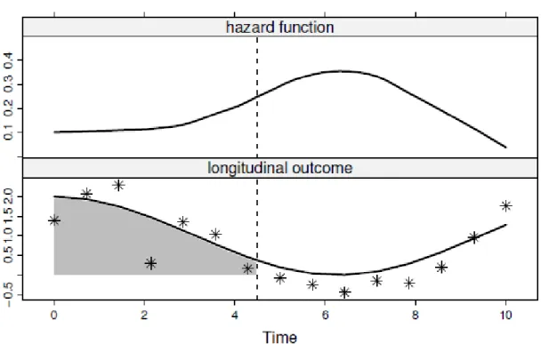
One approach that allows the whole history of the marker to be associated with the hazard for an event is to include the integral of the longitudinal trajectory in the linear predictor of the relative risk submodel, representing the cumulative effect of the longitudinal outcome up to time point t. A graphical representation of this parameterization is given in figure 4. More specifically, the survival submodel takes the form:

where for any particular time point t, α measures the strength of the association between the risk for an event at time point t and the area under the longitudinal trajectory up to the same time t, with the area under the longitudinal trajectory regarded as a suitable summary of the whole trajectory.

To fit a joint model under this parameterization, we can exploit the flexibility provided by the derivForm argument of jointModel() for the specification of an extra marker term to be added in the linear predictor of the survival submodel. In particular, instead of specifying the R formulas to define the time-dependent slope term m′i(t).

Therefore, to arrive at the cJM model in the SPRINT database, the integral of the longitudinal trajectory of SBP was included as the linear predictor of the relative risk sub-model. The

(14)

integral represents the cumulative effect of the longitudinal trajectory of repeated SBP measurements up to time point t. The hazard ratio (HR) for the intensive treatment from the cJM approach, therefore, takes into account the cumulative impact of SBP changes over time.

Figure 4 Graphical concept of cumulative Joint Model for longitudinal and time-to-event data

The top panel illustrates the evolution of the hazard function in time, and the bottom panel shows that at each time point the entire area under the longitudinal trajectory is associated with the hazard.

The command used in R to obtain this cumulative joint model was:

jointFit2_cum <- update(jointFit2, parameterization = "slope", derivForm = iForm2) summary(jointFit2_cum)

exp(confint(jointFit2_cum, parm = "Event"))

(15)

The output with the results of this cumulative joint model are shown below.

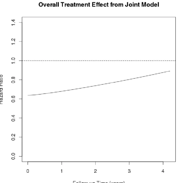
10. Plots of the hazard ratio changes over time for the primary SPRINT outcome We obtained the plots of the changes in the hazard ratios for the primary SPRINT primary outcome over time shown in figure 5. This graph shown us that hazard ratio for intensive

(16)

treatment was losing its protective effect on the primary SPRINT outcome in the total population over time.

Figure 5 Changes in the hazard ratio for intensive treatment on the primary SPRINT outcome in the total population over time

(17)

11. Subgroup analysis based on the original SPRINT subgroups

All of the previous stages were followed in the analysis of the subgroups. We considered the same subgroups as those investigated in the original SPRINT trial. We found the same

tendency regarding losing the protective effect of intensive treatment on the primary SPRINT outcome in subgroup analysis. This was particularly the true for participants with previous chronic kidney disease or cardiovascular disease, women, individuals of Black ethnicity, those younger than 75 year, and participants with SBP >132 mmHg at baseline (Figure 6) Figure 6. Plots of cumulative joint model analysis in the SPRINT subgroups

(18)

12. Subgroup analysis between SAEs vs non-SAEs groups

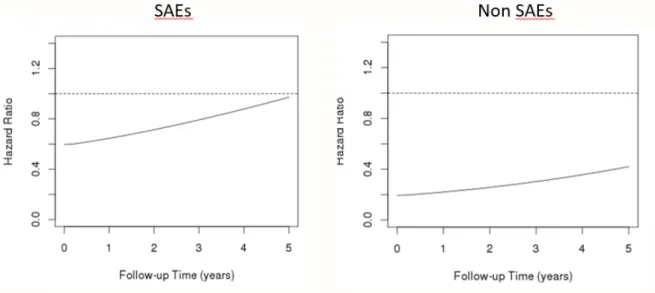
In the cJM, we analyzed the interaction between intensive treatment and SAEs in total population and in each of the subgroups under study and we found statistically significance association (P< 0.0001). Therefore, we stratified the cJM analyses based on occurrence of SAEs during follow-up. We found that the protective effect of intensive treatment in participants who suffered SAEs was lower (higher HR) than non-SAEs participants. At the same time, the protective effect was lost earlier in SAEs participants than non-SAEs participants (Figure 7)

(19)

Figure 7 Plots of cumulative joint model analysis comparing participants with SAEs vs those without SAEs in the SPRINT trial.

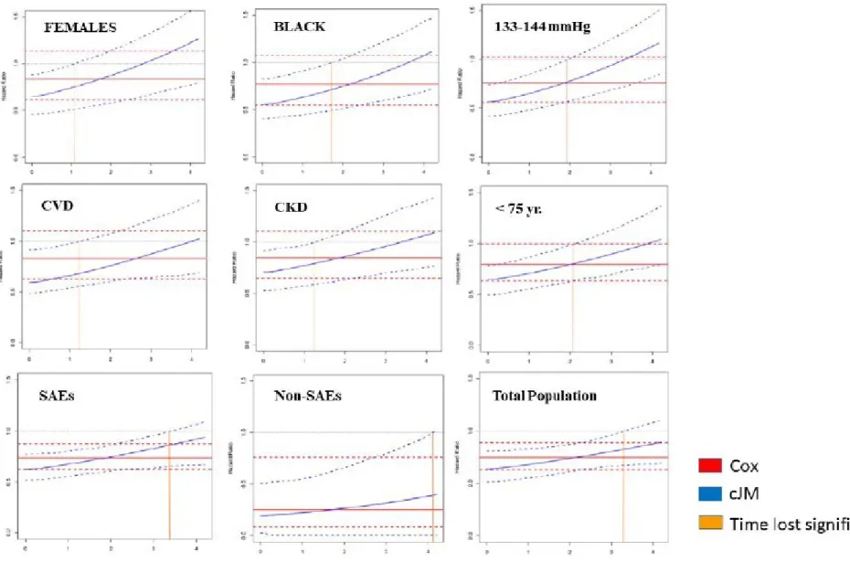
13. Bootstrapping to create summary plots for simultaneous comparison between Cox proportional hazard model and cumulative joint model

Finally, we ran bootstrapping with 400 repetitions in order to obtain the 95% confidence intervals for all plots obtained in our analysis. We included both Cox proportional hazard plots and cumulative joint models in the same graph. In order to facilitate the interpretation of our results, we added an orange vertical line to the graph indicating the time when the

confidence interval of cumulative joint model crossed the level of non-statistical significance (HR=1.0)

All finals plots comparing the changes in the hazard ratio over time using the traditional Cox proportional model versus the cumulative hazard model are shown below. These graphs represent the hazard ratio and 95% confidence interval for intensive systolic blood pressure treatment based on traditional Cox proportional hazard approach (red lines) and cumulative joint model approach (blue lines) for different subgroups: individuals with and without

(20)

ethnicities (E&F); Individuals <75 and >=75 years of age (G&H); individuals with and without prevalent cardiovascular disease at baseline (I&J); baseline systolic blood pressure categories of 133-144 mmHg and <=132mmHg (K&L). Orange vertical line denotes the time point at which the statistical significance of the effect estimate is lost in each subgroup.

(21)

(22)

(23)

14. R software script

###STAGES JOINT MODEL ANALYSIS SBP 1. ### Install packages needed

## Longitudinal data Analysis

install.packages(c("shiny", "nlme", "lattice", "lme4",

"MCMCglmm", "geepack", "MASS", "corrplot", "splines", "Matrix", "md5"), dependencies = TRUE)

library("Rcpp") library("Matrix") library("lme4") library("lattice") library("lme4") library("MASS") library("splines") library("geepack") library("Matrix") library("corrplot") library("MCMCglmm") library("shiny") library("nlme") library("coda") library("ape") library(FinTS) package.dir('nlme')

## Survival Data Analysis install.packages("survival") library("survival")

### Starting second analysis professor Rizopoulos install.packages("JM")

library("JM") library("lattice")

load("Longall_17.RData")

LongData <- Longall_17[c("id", "sbp", "timevisityear", "INTENSIVE", "YEAR_T_PRIMARY",

"EVENT_PRIMARY")]

LongData <- LongData[LongData$timevisityear < LongData$YEAR_T_PRIMARY, ] LongData <- LongData[complete.cases(LongData), ]

LongData <- with(LongData, LongData[order(id, timevisityear), ]) SurvData <- LongData[!duplicated(LongData$id), ]

##########################################################################################

######################################################################################

(24)

plot(survfit(Surv(YEAR_T_PRIMARY, EVENT_PRIMARY) ~ INTENSIVE, data = SurvData)) ids <- sample(LongData$id, 16)

xyplot(sbp ~ timevisityear | id, data = LongData, subset = id %in% ids, type = "b", abline = list(v = 0.25, lty = 2, col = 2))

##########################################################################################

######################################################################################

3. ## Linear mixed model

# account for initial drop in SBP evolution by setting the knots appropriatelly;

# it is also a good idea to set the boundary knots (in this case the upper knot) not to

# the maximum (i.e., the default) but to the 95% percentile of the time variable fm2 <- lme(sbp ~ ns(timevisityear, k = c(0.25, 0.5, 1.4), B = c(0, 3.5)) * INTENSIVE, data = LongData, method = "ML",

random = list(id = pdDiag(form = ~ ns(timevisityear, k = c(0.25, 0.5, 1.4), B = c(0, 3.5))))) summary(fm2)

plot(fm2) qqnorm(fm2)

#######################################################################################

4.## Cox model

CoxFit2 <- coxph(Surv(YEAR_T_PRIMARY, EVENT_PRIMARY) ~ INTENSIVE, data = SurvData, x = TRUE)

summary(CoxFit2)

##########################################################################################

######################################################################################

5.## Standard Joint Model using fm2

jointFit2 <- jointModel(fm2, CoxFit2, timeVar = "timevisityear",

method = "piecewise-PH-aGH", knots = c(0.5, 1, 1.5, 2, 2.5, 3)) summary(jointFit2)

exp(confint(jointFit2, parm = "Event"))

# Overall treatment effect (JM STANDARD POINT)

JMFit <- jointFit2 # select the joint model (only works for jointFit1 & jointFit2) ND1 <- expand.grid(timevisityear = seq(0, 4.2, length.out = 100),

INTENSIVE = 1, sbp = 100, YEAR_T_PRIMARY = 4.2, EVENT_PRIMARY = 1) ND0 <- expand.grid(timevisityear = seq(0, 4.2, length.out = 100),

INTENSIVE = 0, sbp = 100, YEAR_T_PRIMARY = 4.2, EVENT_PRIMARY = 1) fixed1 <- c(model.matrix(JMFit$termsYx, ND1) %*% fixef(JMFit))

fixed0 <- c(model.matrix(JMFit$termsYx, ND0) %*% fixef(JMFit))

(25)

base1 <- c(model.matrix(JMFit$termsT, ND1)[, -1, drop= FALSE] %*% fixef(JMFit, "Event") [c("INTENSIVE")])

alpha <- fixef(JMFit, "Event")["Assoct"]

logHR <- base1 + alpha * fixed1 - base0 - alpha * fixed0 plot(ND1$timevisityear, exp(logHR), type = "l",

ylab = "Hazard Ratio", xlab = "Follow-up Time (years)", main = "Overall Treatment Effect from Joint Model") abline(h = 1, lty = 2)

##########################################################################################

######################################################################################

6. Plots of comparison between LMM model fm1 and model fm2

# check fit of the models in the individual trajectories LongData$fitted1 <- fitted(fm1, level = 1)

LongData$fitted2 <- fitted(fm2, level = 1)

ids <- sample(LongData$id, 16) # a random sample of 16 patients xyplot(sbp + fitted1 + fitted2 ~ timevisityear | id, data = LongData, panel = function (x, y, ...) {

x.mat <- matrix(x, ncol = 3) y.mat <- matrix(y, ncol = 3)

panel.xyplot(x.mat[, 1], y.mat[, 1], type = "p", col = "black") panel.xyplot(x.mat[, 2], y.mat[, 2], type = "l", lwd = 2, col = "blue") panel.xyplot(x.mat[, 3], y.mat[, 3], type = "l", lwd = 2, col = "red") panel.abline(v = 0.25, lty = 2, col = 2)

}, subset = id %in% ids, layout = c(4, 4), as.table = TRUE, xlab = "Time (years)", ylab = "SBP")

##########################################################################################

######################################################################################

7. Cummulative joint model using fm2

## cumulative effect (area) Joint Model using fm2 iForm2 <- list(fixed = ~ 0 + timevisityear

+ ins(timevisityear, k = c(0.25, 0.5, 1.4), B = c(0, 3.5)) + timevisityear:INTENSIVE

+ ins(timevisityear, k = c(0.25, 0.5, 1.4), B = c(0, 3.5)):INTENSIVE, indFixed = seq_along(fixef(fm2)),

random = ~ 0 + timevisityear

+ ins(timevisityear, k = c(0.25, 0.5, 1.4), B = c(0, 3.5)), indRandom = seq_len(ncol(ranef(fm2))))

jointFit2_cum <- update(jointFit2, parameterization = "slope", derivForm = iForm2) summary(jointFit2_cum)

exp(confint(jointFit2_cum, parm = "Event"))

##########################################################################################

######################################################################################

(26)

8. Plots of the hazard ratio changes over time for the SPRINT primary outcome

# Overall treatment effect (JM cumulate)

JMFit <- jointFit2_cum # select the joint model (only works for jointFit1 & jointFit2) ND1 <- expand.grid(timevisityear = seq(0, 4.2, length.out = 100),

INTENSIVE = 0, sbp = 100, YEAR_T_PRIMARY = 4.2, EVENT_PRIMARY = 1) fixed1 <- c(model.matrix(JMFit$termsYx.deriv, ND1) %*% fixef(JMFit)[JMFit$derivForm$indFixed]) fixed0 <- c(model.matrix(JMFit$termsYx.deriv, ND0) %*% fixef(JMFit)[JMFit$derivForm$indFixed]) base1 <- c(model.matrix(JMFit$termsT, ND1)[, -1, drop= FALSE] %*% fixef(JMFit, "Event")

[c("INTENSIVE")])

alpha <- fixef(JMFit, "Event")["Assoct.s"]

logHR <- base1 + alpha * fixed1 - base0 - alpha * fixed0 plot(ND1$timevisityear, exp(logHR), type = "l",

ylab = "Hazard Ratio", xlab = "Follow-up Time (years)",

main = "Overall Treatment Effect from Joint Model", ylim = c(0, 1.4)) abline(h = 1, lty = 2)

########################################################################################

9. Comparison plots between traditional Cox proportional hazard model and cumulative joint model

# Bootstrap CI for overall treatment effect

## bootstrap_cumJM

# Functions

run_boot <- function (m) { library("JM")

load("C:/Users/dimitris/Documents/Students/Oscar/Longall_17.RData") # CHANGE THIS to get data from location on server

LongData <- Longall_17[c("id", "sbp", "timevisityear", "INTENSIVE", "FEMALE", "AGE", "YEAR_T_PRIMARY", "EVENT_PRIMARY")]

LongData <- LongData[LongData$timevisityear < LongData$YEAR_T_PRIMARY, ] LongData <- LongData[complete.cases(LongData), ]

LongData <- with(LongData, LongData[order(id, timevisityear), ]) # function to run model

fit_cumJM <- function (LongData, SurvData) { # Fit cumulative joint model

lmeFit <- lme(sbp ~ ns(timevisityear, k = c(0.25, 0.5, 1.4), B = c(0, 3.5)) * INTENSIVE, data = LongData, method = "ML",

random = list(id_new = pdDiag(form = ~ ns(timevisityear, k = c(0.25, 0.5, 1.4), B = c(0, 3.5)))))

CoxFit <- coxph(Surv(YEAR_T_PRIMARY, EVENT_PRIMARY) ~ INTENSIVE, data = SurvData, x = TRUE)

iForm <- list(fixed = ~ 0 + timevisityear

+ ins(timevisityear, k = c(0.25, 0.5, 1.4), B = c(0, 3.5)) + timevisityear:INTENSIVE

+ ins(timevisityear, k = c(0.25, 0.5, 1.4), B = c(0, 3.5)):INTENSIVE, indFixed = seq_along(fixef(lmeFit)),

random = ~ 0 + timevisityear

+ ins(timevisityear, k = c(0.25, 0.5, 1.4), B = c(0, 3.5)), indRandom = seq_len(ncol(ranef(lmeFit))))

(27)

JMFit <- jointModel(lmeFit, CoxFit, timeVar = "timevisityear",

method = "piecewise-PH-aGH", knots = c(0.5, 1, 1.5, 2, 2.5, 3), parameterization = "slope", derivForm = iForm)

# Overall treatment effect for cumulative effect (area)

ND1 <- expand.grid(timevisityear = seq(0, 4.2, length.out = 100),

INTENSIVE = 0, sbp = 100, YEAR_T_PRIMARY = 4.2, EVENT_PRIMARY = 1)

fixed1 <- c(model.matrix(JMFit$termsYx.deriv, ND1) %*% fixef(JMFit)[JMFit$derivForm$indFixed]) fixed0 <- c(model.matrix(JMFit$termsYx.deriv, ND0) %*% fixef(JMFit)[JMFit$derivForm$indFixed]) base1 <- c(model.matrix(JMFit$termsT, ND1)[, -1, drop= FALSE] %*% fixef(JMFit, "Event")

[c("INTENSIVE")])

alpha <- fixef(JMFit, "Event")["Assoct.s"]

logHR <- base1 + alpha * fixed1 - base0 - alpha * fixed0 exp(logHR)

}

# create Bootstrap sample

create_boot_data <- function (data, idVar, seed = 1L) { set.seed(seed)

ids <- unique(data[[idVar]])

samp_ids <- sample(ids, replace = TRUE) out_data <- vector("list", length(ids)) for (i in seq_along(ids)) {

DD <- data[data[[idVar]] == samp_ids[i], ] DD$id_new <- i

out_data[[i]] <- DD }

rm(list = ".Random.seed", envir = globalenv()) do.call("rbind", out_data)

}

LongData_boot <- create_boot_data(data = LongData, idVar = "id", seed = m) SurvData_boot <- LongData_boot[!duplicated(LongData_boot$id_new), ] # fit joint model and extract results

fit_cumJM(LongData_boot, SurvData_boot) }

##########################################################################################

#####################################################################################

(28)

Supplementary Tables and Figures

Table S1. Hazard Ratio Based on Cumulative Joint Model Approach at the Start and End of Follow-Up in the Total SPRINT Population and among Different Subgroups

cJM (HR CI 95%)

Start Point End point

Total population 0.60 (0.50, 0.72)* 0.89 (0.69, 1.10)

Sub-groups Baseline CKD

CKD 0.75 (0.56, 0.99)* 1.09 (0.76, 1.43)

Non- CKD 0.53 (0.42, 0.68)* 0.91 (0.67, 1.14)

Gender

Female 0.65 (0.47, 0.91)* 1.26 (0.78, 1.61)

Male 0.57 (0.45, 0.71)* 0.91 (0.65, 1.1)

Ethnicity

Black 0.59 (0.40, 0.85)* 1.11 (0.72, 1.47)

Non- black 0.61 (0.49, 0.75)* 0.95 (0.71, 1.15)

Age

< 75 0.67 (0.52, 0.86)* 0.89 (0.79, 1.37)

>= 75 0.56 (0.42, 0.74)* 0.77 (0.59, 1.11)

Baseline CVD

CVD 0.68 (0.50, 0.92)* 1.02 (0.69, 1.4)

Non-CVD 0.57 (0.45, 0.72)* 0.97 (0.74, 1.13)

Baseline SBP

<=132 0.53 (0.38, 0.75)* 0.85 (0.67, 1.34)

133-144 0.57 (0.41, 0.79)* 1.17 (0.85, 1.50)

>= 145 0.70 (0.52, 0.94) * 0.84 (0.70, 1.41)

Serious adverse events

SAEs 0.60 (0.50, 0.72)* 0.94 (0.67, 1.34)

Non-SAEs 0.19 (0.06, 0.63)* 0.40 (0, 1.02)

CI denotes confidence interval, cJM cumulative joint model, CKD chronic kidney disease, CVD cardiovascular disease, HR hazard ratio, SAEs serious adverse events, and SBP systolic blood pressure.

*P < 0.05

(29)

(30)

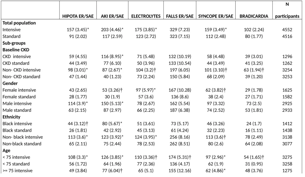
Table S2. Distribution of Specific Serious Adverse Events for the Intensive and Standard Treatment Categories in the Total SPRINT Population and among Different Sub-Groups

HIPOTA ER/SAE AKI ER/SAE ELECTROLYTES FALLS ER/SAE SYNCOPE ER/SAE BRADICARDIA

N participants Total population

Intensive 157 (3.45)* 203 (4.46)* 175 (3.85)* 329 (7.23) 159 (3.49)* 102 (2.24) 4552

Standard 91 (2.02) 117 (2.59) 123 (2.72) 323 (7.15) 112 (2.48) 80 (1.77) 4516

Sub-groups Baseline CKD

CKD intensive 59 (4.55) 116 (8.95)* 71 (5.48) 132 (10.19) 58 (4.48) 39 (3.01) 1296

CKD standard 44 (3.49) 77 (6.10) 50 (3.96) 133 (10.54) 44 (3.49) 41 (3.25) 1262

Non- CKD intensive 98 (3.01)* 87 (2.67)* 104 (3.2)† 197 (6.05) 101 (3.10)† 63 (1.94)† 3254

Non- CKD standard 47 (1.44) 40 (1.23) 73 (2.24) 150 (5.84) 68 (2.09) 39 (1.20) 3253

Gender

Female intensive 43 (2.65) 53 (3.26)† 97 (5.97)* 167 (10.28) 62 (3.82)† 29 (1.78) 1625

Female standard 28 (1.77) 30 (1.9) 57 (3.6) 136 (8.6) 38 (2.4) 27 (1.71) 1582

Male intensive 114 (3.9)* 150 (5.13)* 78 (2.67) 162 (5.54) 97 (3.32) 73 (2.5) 2925

Male standard 63 (2.15) 87 (2.97) 66 (2.25) 187 (6.38) 74 (2.52) 53 (1.81) 2933

Ethnicity

Black intensive 44 (3.12)† 80 (5.67)* 51 (3.61) 73 (5.17) 46 (3.26) 24 (1.7) 1412

Black standard 26 (1.81) 42 (2.92) 45 (3.13) 61 (4.24) 32 (2.23) 16 (1.11) 1438

Non- black intensive 113 (3.6)* 123 (3.92)* 124 (3.95)* 256 (8.16) 113 (3.6)† 78 (2.49) 3138

Non-black standard 65 (2.11) 75 (2.44) 78 (2.53) 262 (8.51) 80 (2.6) 64 (2.08) 3077

Age

< 75 intensive 108 (3.3)* 126 (3.85)* 110 (3.36)† 174 (5.31)† 97 (2.96)* 54 (1.65)† 3275

< 75 standard 56 (1.72) 64 (1.96) 77 (2.36) 136 (4.17) 62 (1.9) 31 (0.95) 3258

>= 75 intensive 49 (3.84) 77 (6.04)† 65 (5.1) 155 (12.16) 62 (4.86)* 48 (3.76) 1275

(31)

>= 75 standard 35 (2.78) 53 (4.22) 46 (3.66) 187 (14.88)† 50 (3.98) 49 (3.9) 1257 Baseline CVD

CVD intensive 44 (4.78)† 60 (6.51)† 47 (5.1)† 76 (8.25) 37 (4.02) 37 (4.02) 921

CVD standard 27 (2.98) 38 (4.2) 26 (2.87) 76 (8.4) 31 (3.43) 26 (2.87) 905

Non-CVD intensive 113 (3.11)* 143 (3.94)* 128 (3.53)† 253 (6.97) 122 (3.36)* 65 (1.79) 3629

Non-CVD standard 64 (1.77) 79 (2.19) 97 (2.69) 247 (6.84) 81 (2.24) 54 (1.5) 3610

Baseline SBP

<=132 intensive 55 (3.57)* 56 (3.63) 31 (2.08) 107 (6.94) 56 (3.63)† 32 (2.08) 1542

<= 132 standard 29 (1.95) 36 (2.42) 57 (3.7)* 97 (6.51) 31 (2.08) 25 (1.68) 1490

133-144 intensive 47 (3.24)* 68 (4.69)* 49 (3.38)† 110 (7.58) 43 (2.96) 34 (2.34) 1451

133-144 standard 26 (1.73) 32 (2.13) 30 (1.99) 115 (7.65) 35 (2.33) 21 (1.4) 1504

>= 145 intensive 55 (3.53) 79 (5.07)† 62 (4.08) 112 (7.19) 60 (3.85) 36 (2.31) 1557

>= 145 standard 36 (2.37) 49 (3.22) 49 (3.38) 111 (7.3) 46 (3.02) 34 (2.24) 1521

CKD: Chronic Kidney Disease; Non-CKD: Non Chronic Kidney Disease; CVD: Cardiovascular Disease; Non-CVD: Non Cardiovascular Disease; SAEs: Serious Adverse Events; Non_SAES: Non Serious Adverse Events.

*P value for the difference between intensive and standard treatment < 0.01

† P value for the difference between intensive and standard treatment < 0.05

(32)

Figure S1. Summary of the main results: Changes in the hazard ratio over time in the SPRINT subgroup that lost early benefits of intensive treatment.

(33)

References

1. Rizopoulos D. Joint Models for Longitudinal and Time-to-Event Data: With Applications in R. 1st ed; 2012.

2. Self, S. and Pawitan, Y. (1992). Modeling a marker of disease progression and onset of disease. In Jewell, N., Dietz, K., and Farewell, V., editors, AIDS, 1992 Epidemiology: Methodological Issues. Birkha¨user, Boston.

3. DeGruttola, V. and Tu, X. Modeling progression of CD-4 lymphocyte count and its relationship to survival time. Biometrics 1994; 50: 1003 – 1014.

4. Faucett, C. and Thomas, D. Simultaneously modelling censored survival data and repeatedly measured covariates: A Gibbs sampling approach.

Statistics in Medicine 1996;15: 1663 – 1685.

5. Wulfsohn, M. and Tsiatis, A. A joint model for survival and longitudinal data measured with error. Biometrics 1997; 53: 330 – 339.

6. Rizopoulos D. JM: An R Package for the Joint Modelling of Longitudinal and Time-to-Event Data. Journal of Statistical Software. 2010;35:1-33.

7. Mauff K, Steyerberg EW, Nijpels G, van der Heijden A, D. Rizopoulos. Extension of the association structure in joint models to include weighted cumulative effects. Statistics in Medicine.

2017; 36:3746-3759.

8. Group SR, Wright JT, Jr., Williamson JD, Whelton PK, Snyder JK, Sink KM, Rocco MV, Reboussin DM, Rahman M, Oparil S, Lewis CE, Kimmel PL, Johnson KC, Goff DC, Jr., Fine LJ, Cutler JA, Cushman WC, Cheung AK and Ambrosius WT. A Randomized Trial of Intensive versus Standard Blood-Pressure Control. N Engl J Med. 2015;373:2103-16.

(34)

9.. Tsiatis A and Davidian M. Joint modeling of longitudinal and time-to-event data: An overview.

Statistica Sinica. 2004;14:809-34.

10. Sylvestre, M.P. and Abrahamowicz, M. Flexible modeling of the cumulative effects of time-dependent exposures on the hazard. Statistics in Medicine. 2009; 28: 3437 – 3453.

11. Hauptmann, M., Wellmann, J., Lubin, J., Rosenberg, P., and Kreienbrock, L. Analysis of exposure-time-response relationships using a spline

weight function. Biometrics. 2000; 56: 1105 – 1108.

12. Vacek, P. Assessing the effect of intensity when exposure varies over time. Statistics in Medicine. 1997; 16: 505 – 513.