SUPPLEMENTARY DATA FOR CHAPTER 2

A p p e n d i x A

SUPPLEMENTARY DATA FOR CHAPTER 2

A.1 General Considerations A.1.1 Chemicals

Toluene, acetonitrile, and diethyl ether were degassed with nitrogen and dried by passage through activated alumina using a solvent purification system. Acetonitrile used in photophysical studies was purchased from Alfa Aesar (HPLC Grade, 99.9%+), degassed by three freeze-pump-thaw cycles, and passed through activated alumina prior to use. Phenyl halides were stored over 4 Å molecular sieves and passed through activated alumina prior to use. The following compounds were synthesized according to literature procedures:

mesitylcopper,¹ 3-methyl-2,3-dihydrobenzofuran,² 1,2-bis(2,6-dimethylphenyl) disulfide,³ 1-(allyloxy)-2-iodobenzene,⁴ 2,6-dimethylphenyl phenyl sulfide,⁵ 2- (allyloxy)benzenediazonium tetrafluoroborate,⁶ [n-Bu4N][B(C6F5)4],⁷ 1-hydroxyl-2,2,6,6- tetramethylpiperidine,⁸ and 1-(but-3-en-1-yloxy)-2-iodobenzene.⁹ All other chemicals were purchased from commercial suppliers.

A.1.2 Infrared, EPR, and UV-Vis Spectroscopy

UV-vis experiments were conducted with sealable 1-cm path length fused quartz cuvettes (Starna Cells) using a Cary 50 UV-vis spectrometer equipped with a UNISOKU Scientific Instruments Coolspek cryostat. X-band EPR measurements were made with a Bruker EMX spectrometer at 77 K. Simulation of EPR data was conducted using EasySpin.¹⁰ IR measurements were recorded on a Bruker ALPHA Diamond ATR.

A.1.3 NMR Spectroscopy

All NMR spectra were obtained at ambient temperature using Varian 400 and 500 MHz spectrometers unless otherwise noted. ¹H NMR chemical shifts (δ) are reported in parts per million (ppm) relative to the proteo solvent impurity (7.26 ppm for CHCl3, 1.94 ppm for CD2HCN). ¹³C NMR chemical shifts were also reported relative to the solvent peak (77.16 for CDCl3).

A.1.4 Mass Spectrometry

The ESI-MS experiment for 2.1 was conducted using a Thermo LCQ ion trap mass spectrometer. Mass spectral data for all organic compounds were collected on an Agilent 5973.

A.1.5 Photophysical Methods

Time-resolved luminescence measurements were conducted using a Q-switched Nd:YAG laser (Spectra-Physics Quanta-Ray PRO-Series) with 8 ns pulses (repetition rate of 10 Hz) in the Beckman Institute Laser Resource Center at the California Institute of Technology. The luminescence was dispersed through a monochromator onto a photomultiplier tube (Hamamatsu R928). Samples were stirred continuously. Steady-state emission spectra were recorded on a Jobin Yvon Spec Fluorolog-3-11. Sample excitation was accomplished with a xenon arc lamp and the right angle emission detected with a photomultiplier tube (Hamamatsu R928P). All measurements were conducted with 1-cm path length fused quartz cuvettes (Starna Cells).

A.1.6 Cyclic Voltammetry

Electrochemical experiments were performed in acetonitrile with 0.1 M [n- Bu4N][B(C6F5)4] as the electrolyte in a nitrogen-filled glovebox. A CH 600B potentiostat was used with a glassy carbon working electrode and a platinum wire auxiliary electrode.

The reference electrode was a Ag/AgNO3 (0.1 mM)/acetonitrile reference electrode (also contained 0.1 M [n-Bu4N][B(C6F5)4]) separated from the solution by a Vycor frit. The reference electrode was externally referenced to ferrocene. All reported potentials were determined against the reference electrode and converted to SCE by adding 380 mV.

A.1.7 Photolytic Reactions

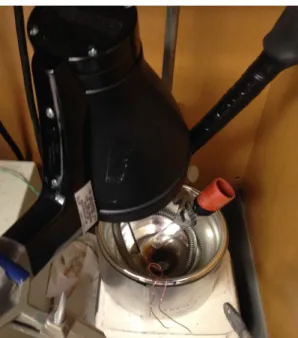
Photolytic reactions were performed using a 100-W Blak-Ray Long Wave Ultraviolet Lamp (Hg), 100-W Blak-Ray B-100Y High Intensity Inspection Lamp (Hg), or a Luzchem LZC-4V photoreactor equipped with LZC-UVA lamps centered around 350 nm.

Temperature control was maintained with either an ice water bath, or isopropanol bath cooled by an SP Scientific cryostat. For reactions using mercury lamps, the light source was placed approximately 20 cm above the sample and the reaction mixture was stirred vigorously using a magnetic stir bar. All reactions were performed in VWR 16 x 100 mm borosilicate culture tubes that were capped with septa and electrical tape. Punctures in the septa were sealed with vacuum grease.

Figure A.1: Representative example of reaction setup using a 100-W Hg lamp. Ice is excluded for clarity.

A.1.8 Chromatography

Normal phase column chromatography was performed using Silicycle 230-400 mesh silica gel. Analytical thin layer chromatography was conducted with Merck aluminum- backed TLC plates (silica gel 60 F254) and plates were visualized under UV light. Reverse- phase chromatography was performed with a Biotage Isolera Spektra Four system.

A.1.8 Other Characterization Methods

Elemental analysis was performed by Midwest Microlab, LLC. Calibrated GC yields were obtained using an Agilent 6890N gas chromatograph (FID detector) with dodecane as an internal standard.

A.1.9 X-ray Crystallography

XRD studies were carried out at the Beckman Institute Crystallography Facility on a Bruker D8 Venture kappa duo photon 100 CMOS instrument (Mo Kα radiation). Structures

were solved using SHELXT and refined against F² by full-matrix least squares with SHELXL and OLEX2. Hydrogen atoms were added at calculated positions and refined using a riding model. The crystals were mounted on a glass fiber or a nylon loop with Paratone N oil.

A.2 Synthesis and Characterization Reported yields have not been optimized.

General Procedure A: This procedure is a modification of that developed by Peters, Fu, and co-workers.⁵ In a nitrogen-filled glovebox, electrophile, NaOt-Bu, CuI, and acetonitrile were added to a borosilicate tube. The tube was then capped with a septum and sealed with electrical tape. On a Schlenk line, 2,6-dimethylthiophenol was added via syringe.

The vessel was then immersed in a cooling bath and irradiated for the specified period. The reaction mixture was then concentrated and the crude material extracted in diethyl ether and filtered through a thin pad of silica. Following concentration, the material was purified by column chromatography.

General Procedure B: The method developed by Venkataraman and coworkers was used for the synthesis of the following compounds.^{10, 11} In a nitrogen-filled glovebox, a borosilicate test tube or round bottom flask was charged with CuI (10 mol%), neocuproine (DMPHEN) or its hemihydrate (10 mol%), aryl iodide (1 equiv.), NaOt-Bu (1.5 equiv.), and toluene. The reaction vessel was removed from the glovebox and connected to a Schlenk line. The reaction mixture was charged with 2,6-dimethylthiophenol (1.1 equiv.) via syringe.

The reaction mixture was heated at 105 to 110 °C for the specified time, cooled to room temperature, and filtered. The crude material was purified by column chromatography.

Copper(I) bis(2,6-dimethylthiophenolate) sodium bis(12- crown-4) ([Cu^I(SAr)2]Na) A Schlenk bomb was charged with NaOt-Bu (90.7 mg, 0.943 mmol), mesitylcopper (181 mg, 0.991 mmol), and acetonitrile (4 mL) in the glovebox. The bomb was removed from the glovebox and connected to a Schlenk line. 2,6-dimethylthiphenol (250 µL, 1.88 mmol) was added via syringe, causing the orange suspension to turn white. The reaction mixture was stirred for 30 min at which time the bomb was returned to the glovebox and it contents filtered through a plug of Celite. 12-crown-4 (162 µL, 1.00 mmol) was added to the filtrate, inducing precipitation of a white solid. The supernatant was removed via pipette and the solid washed with diethyl ether. The desired product was isolated as an analytically pure white solid (214 mg, 0.300 mmol, 32% yield) following removal of solvent in vacuo. X-ray quality crystals were grown from an acetonitrile solution at ambient temperature over 12 h.

1H NMR (400 MHz, CD3CN): δ 6.91 (d, J = 7.4 Hz, 4H), 6.70 (t, J = 7.4 Hz, 2H), 3.62 (s, 32H), 2.42 (s, 12H). HR-MS (ESI) (m/z) calcd for [C16H18CuS2]^–: 337.0146, found:

337.1133. Calculated for C32H50CuNaO8S2: C, 53.88; H, 7.06. Found: C, 53.69, H, 7.14. UV- vis (MeCN): λmax = 258 nm, ε = 2.3 × 10⁴ M^-1 cm^-1.

Sodium 2,6-dimethylthiophenolate A Schlenk flask was charged with oil-free sodium hydride (175 mg, 7.29 mmol) and diethyl ether (20 mL) in the glovebox and the vessel sealed with a septum. The reaction mixture was cooled to 0 °C and 2,6- dimethylthiophenol (1.00 mL, 7.51 mmol) delivered to the suspension via syringe on a Schlenk line. White precipitate immediately formed. Following stirring for 48 h at ambient

SNa S Cu

S [Na(12-crown-4)₂]

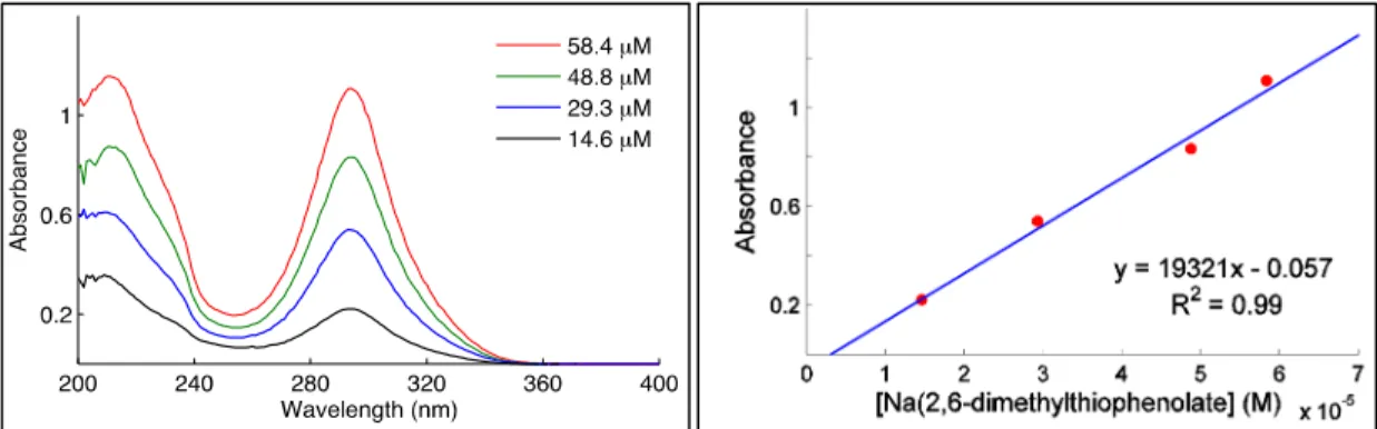
temperature, the solvent was cannulated from the flask and the solid triturated with pentane (ca. 100 mL). The desired product was isolated as a spectroscopically pure white solid (1.05 g mg, 6.52 mmol, 89% yield) following removal of solvent in vacuo. ¹H NMR (400 MHz, CD3CN) δ 6.80 (d, J = 7.3 Hz, 2H), 6.44 (t, J = 7.5 Hz, 1H), 2.30 (s, 6H).UV-vis (MeCN):

λmax = 292 nm, ε = 1.9 ×10⁴ M^-1 cm^-1.

4-Methoxyphenyl 2,6-dimethylphenyl sulfide According to General Procedure B, CuI (42.0 mg, 0.22 mmol), DMPHEN hemihydrate (43.6 mg, 0.20 mmol), 4-iodoanisole (463 mg, 1.98 mmol), 2,6-dimethylthiophenol (280 µL, 2.21 mmol), toluene (6 mL) and NaOt-Bu (293 mg, 3.05 mmmol) were heated for 48 h. The product was isolated as a white solid (251 mg, 1.03 mmol, 52% yield) following column chromatography (SiO2, 4%

EtOAc:hexanes). ¹H NMR (400 MHz, CDCl3): δ 7.23 – 7.12 (m, 3H), 6.91 (d, J = 8.7 Hz, 2H), 6.75 (d, J = 8.7 Hz, 2H), 3.75 (s, 3H), 2.43 (s, 6H). ¹³C NMR (101 MHz, CDCl3): δ 157.6, 143.6, 132.0, 129.0, 128.7, 128.5, 128.0, 114.8, 55.4, 22.1. LR-MS (EI) (m/z) calculated for [C15H19OS]⁺: 244.1, found: 244.1. FT-IR (thin film): 3059, 2954, 2832, 1592, 1572, 1490, 1459, 1439, 1283, 1238, 1173, 1032, 820, 769, 638, 625, 536, 507 cm^-1.

2-(Allyloxy) 2,6-dimethylphenyl sulfide According to General Procedure B, CuI (19.3 mg, 0.10 mmol), DMPHEN hemihydrate (22.1 mg, 0.10 mmol), 1-(allyloxy)-2-iodobenzene (251 mg, 0.96 mmol), 2,6-dimethylthiophenol (140 µL, 1.10 mmol), toluene (6 mL) and NaOt-Bu (147 mg, 1.5 mmmol) were heated for 14 h. The product was isolated as a white solid (178 mg, 0.658 mmol, 69% yield) by column chromatography (SiO2, 4% EtOAc:hexanes).¹H NMR (400 MHz, CDCl3) δ 7.30 – 7.14 (m, 3H), 7.07 – 6.97 (m,

S O MeO

S

1H), 6.84 (d, J = 8.1 Hz, 1H), 6.72 (td, J = 7.6, 1.2 Hz, 1H), 6.33 (dd, J = 7.8, 1.6 Hz, 1H), 6.11 (ddt, J = 17.4, 10.3, 5.0 Hz, 1H), 5.51 (dq, J = 17.3, 1.7 Hz, 1H), 5.32 (dq, J = 10.6, 1.6 Hz, 1H), 4.67 (dt, J = 5.1, 1.7 Hz, 2H), 2.42 (s, 6H). ¹³C NMR (101 MHz, CDCl3): δ 154.6, 144.5, 133.3, 129.8, 129.3, 128.6, 127.1, 125.2, 124.9, 121.6, 117.6, 112.1, 69.6, 21.9. LR- MS (EI) (m/z) calculated for [C17H18OS]⁺: 270.1, found: 270.1. FT-IR (thin film): 3059, 3017, 2955, 2920, 2894, 1575, 1474, 1439, 1233, 1103, 1040, 994, 919, 767, 742 cm^-1.

3-(2,6-dimethylphenylthiomethyl)-2,3-dihydrobenzo-furan According to General Procedure A, CuI (15.7 mg, 0.082 mmol), NaOt-Bu (76.5 mg, 0.796 mmol), 1-(allyloxy)-2-iodobenzene (208 mg, 0.800 mmol), 2,6-dimethylthiophenol (102 µL, 0.800 mmol), and acetonitrile (2.5 mL) were combined and photolyzed with a mercury lamp for 19 h at –20 °C. The reaction mixture was concentrated, and the resulting material suspended in diethyl ether and filtered to remove insoluble byproducts. The product was isolated as a pale yellow oil (96.6 mg, 0.358 mmol, 45% yield) by column chromatography on silica gel (0  2% EtOAc/hexanes), followed by column chromatography using reverse-phase C-18 silica gel (0  100% acetonitrile/water). Due to coelution of the title compound and its uncylized isomer despite multiple attempts at purification, < 2% of the contaminant is detectable by GC and ¹H NMR analysis. ¹H NMR (400 MHz, CDCl3): δ 7.19 (d, J = 7.4 Hz, 1H), 7.13 (m, 4H), 6.85 (td, J = 7.4, 1.0 Hz, 1H), 6.79 (d, J = 8.0 Hz, 1H), 4.63 (t, J = 9.0 Hz, 1H), 4.45 (dd, J = 9.1, 5.8 Hz, 1H), 3.63 – 3.45 (m, 1H), 3.06 (dd, J = 12.6, 4.6 Hz, 1H), 2.75 (dd, J = 12.7, 10.0 Hz, 1H), 2.56 (s, 6H). ¹³C NMR (101 MHz, CDCl3): δ 160.0, 143.0, 133.0, 129.4, 128.9, 128.5, 128.4, 124.5, 120.6, 109.9, 76.3, 42.6, 39.9, 22.2. LR-MS (EI) (m/z) calculated

O S

for [C17H18OS]⁺: 270.1, found: 270.1. FT-IR (thin film): 3056, 2952, 2923, 2877, 1582, 1488, 1459, 1221, 1023, 772, 753 cm^-1.

2-(but-3-en-yloxy) 2,6-dimethylphenyl sulfide According to General Procedure B, CuI (20.9 mg, 0.11 mmol), DMPHEN (11.0 mg, 0.0528 mmol), 1-(but-3-en-1-yloxy)-2-iodobenzene (136 mg, 0.990 mmol), 2,6-dimethylthiophenol (140 µL, 0.496 mmol), toluene (3 mL) and NaOt-Bu (73.2 mg, 0.761 mmmol) were heated for 16 h. The product was isolated as a colorless oil (101 mg, 0.354 mmol, 54% yield) following column chromatography (SiO2, 1  2% EtOAc/hexanes). ¹H NMR (400 MHz, CDCl3) δ 7.34 – 7.18 (m, 3H), 7.07 (ddd, J = 8.0, 7.3, 1.6 Hz, 1H), 6.88 (dd, J = 8.1, 1.3 Hz, 1H), 6.75 (td, J = 7.5, 1.2 Hz, 1H), 6.40 (dd, J = 7.7, 1.6 Hz, 1H), 6.04 (ddt, J = 17.0, 10.2, 6.8 Hz, 1H), 5.35 – 5.12 (m, 2H), 4.17 (t, J = 6.8 Hz, 2H), 2.68 (qt, J = 6.8, 1.4 Hz, 2H), 2.47 (s, 6H). ¹³C NMR (101 MHz, CDCl3) δ 154.9, 144.3, 134.5, 129.9, 129.2, 128.5, 127.0, 125.3, 124.9, 121.4, 117.2, 111.8, 68.3, 33.8, 21.8. LR-MS (EI) (m/z) calculated for [C18H20OS]⁺: 284.1, found: 284.3.

FT-IR (thin film): 3058, 2922, 1576, 1462, 1441, 1237, 1041, 1027, 918, 771, 743 cm^-1.

O S

4-(methylchromane) 2,6-dimethylphenyl sulfide According to General Procedure A, CuI (9.0 mg, 0.047 mmol), 1-(allyloxy)-2- iodobenzene (122 mg, 0.445 mmol), 2,6-dimethylthiophenol (66.0 µL, 0.496 mmol), and NaOt-Bu (47.0 mg, 0.489 mmol) in acetonitrile (5 mL) were photolyzed with 350 nm light in a photobox at ambient temperature for 18 h. The product was isolated as a colorless semi-solid (24.0 mg, 0.084 mmol, 19% yield) by column chromatography on silica gel (0  2% EtOAc/hexanes), followed by column chromatography using reverse-phase C-18 silica gel (0 to 100%

acetonitrile/water). ¹H NMR (400 MHz, CDCl3): δ 7.14 (ap s, 3H), 7.09 (tdd, J = 7.3, 1.9, 0.6 Hz, 2H), 7.02 – 6.94 (m, 1H), 6.88 – 6.73 (m, 1H), 4.30 – 4.20 (m, 1H), 4.20 – 4.09 (m, 1H), 3.12 – 3.04 (m, 1H), 2.96 – 2.87 (m, 1H), 2.88 – 2.79 (m, 1H), 2.59 (d, J = 0.7 Hz, 6H), 2.31 – 2.23 (m, 1H), 2.22 – 2.08 (m, 1H). ¹³C NMR (101 MHz, CDCl3): δ 154.6, 142.8, 133.6, 129.2, 128.2, 127.8, 124.7, 120.3, 116.9, 62.9, 41.7, 33.9, 26.0, 22.1. LR-MS (EI) (m/z) calculated for [C18H20OS]⁺: 284.1, found: 284.4. FT-IR (thin film): 3052, 2951, 2919, 1596, 1480, 1459, 1230, 965, 771, 747 cm^-1.

2-(2,6-dimethylphenylthio)-benzophenone According to General Procedure B, CuI (20.9 mg, 0.11 mmol), DMPHEN hemihydrate (21.7 mg, 0.10 mmol), 2-iodobenzophenone (305 mg, 0.990 mmol), 2,6-dimethylthiophenol (140 µL, 1.10 mmol), toluene (6 mL), and NaOt-Bu (143 mg, 1.5 mmmol) were heated for 20 h. The product was isolated as a white solid (170 mg, 0.534 mmol, 54% yield) by column chromatography (SiO2, hexanes). ¹H NMR (400 MHz, CDCl3): δ 7.86 (d, J = 6.8 Hz, 2H), 7.61 (t, J = 7.4 Hz, 1H),

O S

O S

7.54 – 7.46 (m, 2H), 7.44 (d, J = 7.6 Hz, 1H), 7.25 – 7.06 (m, 5H), 6.68 (d, J = 8.0 Hz, 1H), 2.38 (s, 6H). ¹³C NMR (101 MHz, CDCl3): δ 196.7, 144.0, 139.7, 137.7, 136.2, 133.1, 131.3, 131.0, 130.6, 130.3, 129.5, 128.6, 128.5, 126.3, 123.9, 21.9. LR-MS (EI) (m/z) calculated for [C21H18OS]⁺: 318.1, found: 318.1. FT-IR (thin film): 3057, 2972, 2949, 2919, 1656 (C=O), 1597, 1580, 1462, 1432, 1315, 1284, 1254, 924, 762, 742, 699, 638 cm^-1.

A.3 Molar Conductivity Measurements

Conductivity measurements were made using a VWR SB80PC sympHony Meter and conductivity probe. The meter was calibrated using aqueous NaCl solutions. All measurements were made using 1 mM solutions of analyte in acetonitrile at 21 °C and corrected to 25 °C using a linear correction of 2.1% per °C.

Table A.1: Molar conductivities of measured compounds.

Compound Λ_m (S cm² mol^-1)

Ferrocene 0.45

[TBA][PF6] 168.1

2.1 128.5

A.4 Spectroscopic Identification of Copper(II) Species

Identification by UV-vis. Using propionitrile stock solutions to deliver each reagent, solutions of [Cu^I(SAr)2]Na (4. 6 mM, 1 mL, 4.6 µmol), PhI (49 mM, 0.5 mL, 24.5 µmol), and sodium 2,6-dimethylthiophenolate (24 mM, 1 mL, 24.0 µmol) were transferred to a cuvette in a nitrogen-filled glovebox. The reaction mixture was diluted with additional propionitrile (1.5 µM in [Cu^I(SAr)2]Na), and the cuvette sealed with a Teflon valve and brought ou;tside of the glovebox. The vessel was cooled to -78 °C and irradiated with a 100- W Hg lamp for 5 min resulting in a blue solution. The cuvette was quickly transferred to the cooled UV-vis cryostat (-80 °C) and the spectrum collected. Control experiments were

prepared identically but with exclusion of one or more components and dilution to a total volume of 3 mL.

Identification by EPR. The model complex [Cu^I(SAr)2]Na (7.0 mg, 0.010 mmol), sodium 2,6-dimethylthiophenolate (8.2 mg, 0.051 mmol), and iodobenzene (0.070 mmol) were diluted in 1:1 propionitrile:butyronitrile (2 mL). An aliquot of the solution was transferred to an EPR tube and sealed. Outside of the glovebox, the tube was irradiated with a 100-W Hg lamp for 5 min at -78 °C. The sample was immediately transferred to a liquid nitrogen-filled dewar and analyzed by EPR spectroscopy. Control experiments were prepared identically but with exclusion of one or more components.

A.5 Identification of 2.1 by ESI-MS

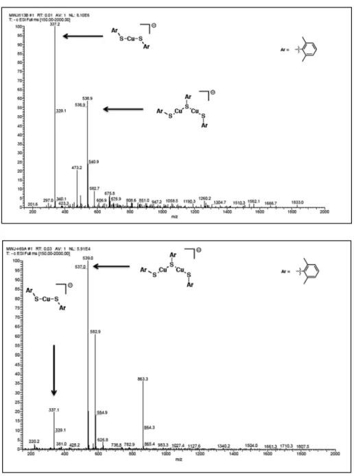
To a borosilicate tube in a nitrogen-filled glovebox was added, sequentially, CuI (6.3 mg, 0.033 mmol), NaOt-Bu (31.9 mg, 0.33 mmol), iodobenzene (37 µL, 0.33 mmol), and acetonitrile (1 mL). The vessel was fitted with a septum and removed from the glovebox.

2,6-dimethyl thiophenol (44 µL, 0.33 mmol) was added via syringe. The heterogeneous reaction mixture was stirred at 0 °C for 1 h under continuous illumination by a 100-W Hg lamp. An aliquot was drawn via a syringe equipped with a filter, and the sample diluted in acetonitrile. Subsequently, the sample was analyzed by ESI-MS.

Figure A.2: ESI-MS of 2.1. Generated during catalysis (top) and independently synthesized (bottom).

A.6 Radical Clock Experiments

All reaction mixtures were analyzed for coupled cyclized product, uncyclized coupled product, starting material, protodehalogenated starting material, and cyclized

protodehalogenated product. Yields were determined by GC with the assistance of dodecane as an internal standard.

Stoichiometric Reaction 2.1 with Radical Clocks. In a nitrogen filled glovebox, a borosilicate test tube was charged with 2.1 (7.1 mg, 0.010 mmol), electrophile (0.010 mmol), and acetonitrile (0.02 M). The reaction mixture was photolyzed for 5 h at which time it was diluted with diethyl ether and dodecane was added (0.010 mmol). The mixture was filtered through silica and analyzed by GC.

Table A.2: Reactivity of 2.1 with 1-(allyloxy)-2-iodobenzene.

Run 1 2% 50% 0% 4% 38%

Run 2 2% 46% 0% 4% 44%

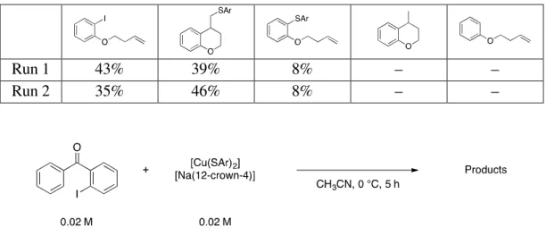
Table A.3: Reactivity of 2.1 with 1-(but-3-en-1-yloxy)-2-iodobenzene.

Run 1 43% 39% 8% – –

Run 2 35% 46% 8% – –

Table A.4: Reactivity of 2.1 with 2-iodobenzophenone.

Run 1 46 0% 8% 0% 11%

Run 2 41 0% 4% 0% 23%

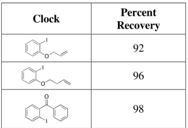
Determination of Radical Clock Stability. All radical clocks were subjected to the same conditions as in the stoichiometric reaction (vide supra) but in the absence of [Cu^I(SAr)2]Na.

Table A.5: Stability of radical clocks.

Clock Percent

Recovery 92 96

98

A.7 Stoichiometric of [Cu^I(SAr)2]Na with Phenyl Halides

All reaction mixtures were analyzed for product, unreacted phenyl halide, biphenyl, and succinonitrile. Yields were determined by GC with the assistance of dodecane as an internal standard.

Stoichiometric Reaction of 2.1 with Phenyl Halides. In a nitrogen filled glovebox, a borosilicate test tube was charged with 2.1 (7.1 mg, 0.010 mmol), electrophile (0.010 mmol), and acetonitrile (0.02 M). The reaction mixture was photolyzed for 5 h at which time it was diluted with diethyl ether and dodecane was added (0.010 mmol). The mixture was filtered through silica and analyzed by GC.

Table A.6: Reactivity of 2.1 with iodobenzene and control experiments.

Run 1 (% yeld) Run 2 (%

yield)

PhI 54 57

No light 0 0

No light or catalyst 0 0

A.8 Stern-Volmer Quenching Experiment

Stern-Volmer Kinetic Analysis. Complex 2.1 (30.1 mg, 0.0422 mmol) was diluted in acetonitrile (10 mL, 4.22 mM). Iodobenzene (618 mg, 3.03 mmol) was diluted in acetonitrile (10 mL, 303 mM). An acetonitrile solution of 2.1 (1.2 mM) was prepared with varying amounts of iodobenzene solution. Data were analyzed using Matlab R2015A with the default curve fitting function.

Table A.7: Excited-state lifetime as a function of quencher concentration.

Concentration of PhI (mM) Lifetime (µs)

0 6.8

43.3 6.0

86.6 4.6

130 4.0

173 3.6

A.9 Steady-State Fluorimetry Experiment

Emission and Excitation of 2.1. A 25 µM solution of 2.1 in acetonitrile was excited using a Xe arc lamp (425 W) at 353 nm and the right angle emission detected at 675 nm. A 470 nm long-pass filter was used in determining both the excitation maximum and minimum.

A.10 Reactivity of 1-(but-3-en-1-yloxy)-2-iodobenzene with [Cu^I(SAr)2]Na

A stock solution of 1-(but-3-en-1-yloxy)-2-iodobenzene (1.0 mL, 0.010 M, 0.010 mmol) was added to a borosilicate tube containing [Cu^I(SAr)2]Na. The reaction mixtures were photolyzed at 0 °C for 5 h with a mercury lamp. The reaction mixtures were then passed through a plug of silica diluted with ether, and the product distribution determined by GC.

Table A.8: Product distribution in the reaction of 2.1 with 1-(but-3-en-1-yloxy)-2- iodobenzene.

[Cu^I(SAr)2]Na

(mmol) Yield X (%) Yield Y (%) Ratio

1.0 6.8 31 4.6

1.5 9.3 39 4.2

2.0 5.9 23 3.9

2.5 9.6 44 4.6

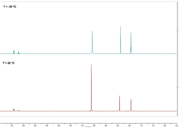
A.11 VT-NMR Study of 2.1

The ¹H NMR spectrum of 2.1 in CD3CN (5 mM) was collected at 22 °C (bottom).

The sampled was cooled to –30 °C in the probe and an additional spectrum collected.

Figure A.3: Low temperature (–30 °C, center) and ambient temperature (22 °C, bottom) ¹H NMR of 2.1.

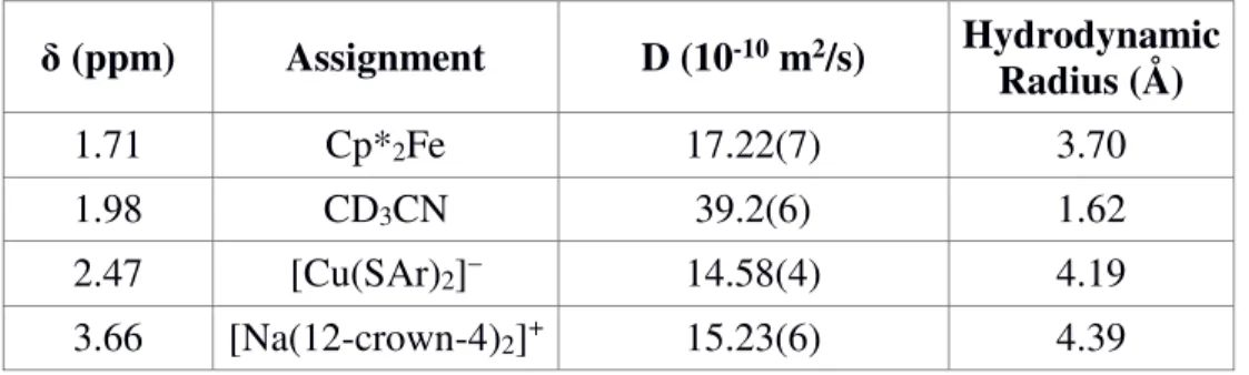
A.12 DOSY Experiment

DOSY Procedure. [Cu^I(SAr)2]Na (5 mg, 7 µmol) and decamethylferrocene (0.3 mg, 0.9 µmol) were weighed into an NMR tube, and CD3CN (0.5 mL) was added. A DOSY spectrum was acquired on a Varian 500 MHz spectrometer with a probe temperature of 25.0

°C, and the diffusion constants were calculated by exponential fit to the individual spectra.

Hydrodynamic radii were calculated from the diffusion constants using the Stokes-Einstein equation.

Table A.9: Measured Hydrodynamic Radii.

δ (ppm) Assignment D (10^-10 m²/s) Hydrodynamic Radius (Å)

1.71 Cp*2Fe 17.22(7) 3.70

1.98 CD3CN 39.2(6) 1.62

2.47 [Cu(SAr)2]^– 14.58(4) 4.19

3.66 [Na(12-crown-4)2]⁺ 15.23(6) 4.39

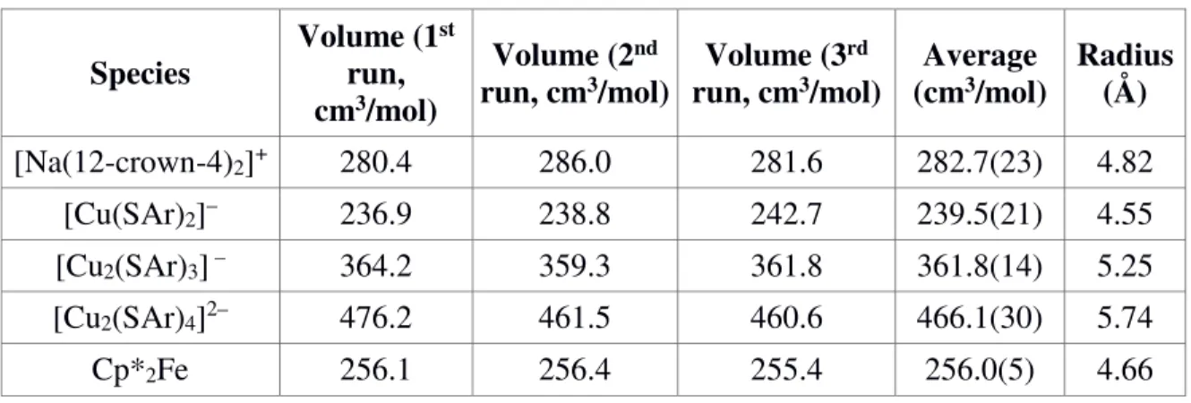
Calculation of Molar Volumes. Molar volumes were calculated from the DFT- optimized geometries. In Gaussian 09, a single point calculation was run using the BP86 functional and def2-TZVP basis set for all atoms. The molar volume was then calculated by Monte-Carlo integration over the electron density grid (‘Volume’ keyword, 0.001 e-/Bohr³ cutoff density, 1000 test points/Bohr³). All volume calculations were run in triplicate due to the random error associated with Monte-Carlo methods.

Table A.10: DFT-Calculated Radii.

Species Volume (1^st run, cm³/mol)

Volume (2^nd

run, cm³/mol) Volume (3^rd

run, cm³/mol) Average

(cm³/mol) Radius (Å) [Na(12-crown-4)2]⁺ 280.4 286.0 281.6 282.7(23) 4.82

[Cu(SAr)2]^– 236.9 238.8 242.7 239.5(21) 4.55 [Cu2(SAr)3] ^– 364.2 359.3 361.8 361.8(14) 5.25 [Cu2(SAr)4]^2– 476.2 461.5 460.6 466.1(30) 5.74

Cp*2Fe 256.1 256.4 255.4 256.0(5) 4.66

A.13 Actinometric Studies

Determination of light intensity. All actinometric experiments were conducted in a Jobin Yvon Spec Fluorolog-3-11 fluorimeter with a 425 W Xe arc lamp using an excitation

wavelength of 365 nm and an excitation slit width of 10 nm. The fluorimeter lamp was allowed to warm up for at least one hour prior to irradiation of samples. The photon flux of the fluorimeter was determined by ferrioxalate actinometry using the method of Bolton,¹² using a quantum yield of 1.28 for ferrioxalate reduction.¹³ Solutions were irradiated for 0, 20, 40, and 60 seconds, and the quantum yield was determined for each sample. A photon flux of 2.9(3) * 10^-8 einsteins s^-1 was calculated by averaging all time points.

Sample photon flux calculation for 20 second photolysis:

= ∗ 10 ∗

1000 ∗ ∗ = 3.0 ∗ 10 ∗ 0.28

1.0 ∗ 1000 ∗ 11,100

= 7.5 ∗ 10

ℎ ! "# =

$ℎ% ∗ ∗ ! = 7.5 ∗ 10

1.28 ∗ 20 = 2.9 ∗ 10 ^' % ( % ( (

Where V1 is the volume irradiated, V is the aliquot volume, and ε is the extinction coefficient of the Fe(II) phenanthroline complex.

Determination of quantum yield for stoichiometric model reaction. To a 1-cm cuvette with a Kontes valve or screw cap was added [Cu^I(SAr)2]Na (0.06 mmol, 1 equiv), PhI (0.06 mmol, 1 equiv), and MeCN (3.0 mL). A stir bar was added, and the cuvette was sealed. The absorbance of the solution at 365 nm was measured by UV-vis prior to irradiation. The sample was cooled to 0 °C and placed in a cuvette holder cooled to 0 °C with an internal cooling loop. While stirring, the sample was irradiated for one hour. The absorbance of the solution at 365 nm was measured by UV-vis following irradiation. After

irradiation, Et2O (3 mL) and dodecane (0.06 mmol, 1 equiv) was added. The resulting mixture was passed through a silica plug and was analyzed by GC.

The fraction of light absorbed by the solutions at 365 nm was determined by taking the average between the absorbance prior to irradiation and post irradiation. This was converted to fraction of light absorbed (f), where A is the average absorbance.

! = 1 – 10 ^*

The quantum yield of the reaction was then determined using the following equation:

+ = ℎ ! "# ∗ ∗ !

The reported quantum yield of 0.08 is the average of two experiments that gave quantum yields of 0.079 and 0.074.

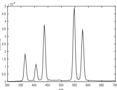
A.14 Emission Spectrum of 100-W Hg Lamp

The emission spectrum was measured using a J & M Analytik TIDAS S 300 K detector.

Figure A.4: Emission spectrum of 100-W Blak-Ray Long Wave Ultraviolet Lamp (Hg).

A.14 Determination of Molar Absorptivities (ε)

Figure A.5: Absorbance spectra of [Cu^I(SAr)2]Na in acetonitrile at various concentrations (left). Absorbance at 258 nm as a function of concentration (right).

nm

300 350 400 450 500 550 600 650 700

Counts

×10⁴

0 0.5 1 1.5 2 2.5 3 3.5 4 4.5 5

[2.1] (M)

Figure A.6: Absorbance spectra of sodium 2,6-dimethylthiophenolate in acetonitrile at various concentrations (left). Absorbance at 292 nm as a function of concentration (right).

A.15 Absorption Spectra of 2.1 in the Presence of NaSAr

UV-Vis Spectra of [Cu^I(SAr)2]Na in Varying Concentrations of Sodium 2,6- Dimethylthiophenolate. A propionitrile solution of [Cu^I(SAr)2]Na (30 µM, 2.5 mL) was added to a septum-sealed cuvette and its spectrum collected. A propionitrile solution of NaSAr (8.1 mM) was added in 20-µL volumes via syringe to the cuvette and the spectrum of the resulting solution collected.

Figure A.7: Optical spectra of 2.1 in the presence of increasing concentrations of sodium 2,6-dimethylthiophenolate.

UV-Vis Spectra of [Cu^I(SAr)2]Na at Various Temperatures in the Presence of Sodium 2,6-Dimethylthiophenolate. A propionitrile solution of [Cu^I(SAr)2]Na (30 µM) in the presence of sodium 2,6-dimethythiophenolate (80 µM) was cooled from 25 to –80 °C and the spectrum collected in 20-degree intervals.

Figure A.8: Optical spectra of 2.1 in the presence of sodium 2,6-dimethylthiophenolate at variable temperature.

A.16 DFT Calculations

General Considerations. The Orca 3.0.1 program was used for all calculations.¹⁴ All optimizations and energy calculations were conducted with tight convergence criteria using the BP86 functional and def2-TZVP basis set,^{15, 16} with the def2-TZVP effective core potential used for iodine.¹⁷ Open and closed shell species were modeled within the unrestricted and restricted Kohn-Sham formalisms, respectively. When energies were compared between open- and closed-shell species, the unrestricted Kohn-Sham formalism was used for all species. All geometry optimizations were conducted without symmetry constraints using gradient methods. Ground state geometries were verified as true minima by the absence of imaginary frequencies. All energies reported are Gibbs free energies at 298.15

K which include translational, rotational, vibrational, and solvation energy contributions.

Solvation was treated with the conductor-like screening model, using default parameters for acetonitrile in all cases.

Figure A.9: Calculated free energies of two possible Cu(I) speciations.

Figure A.10: Calculated free energies of three possible Cu(II) speciations.

Table A.11: Free energies of computed molecules.

Compound Gibbs Free Energy

(Hartrees) [2,6-dimethylthiophenolate] ^– –708.6642 [Cu(2,6-dimethylthiophenolate)2] ^– –3058.0630 [Cu(2,6-dimethylthiophenolate)3]^2– –3766.6958 Cu(2,6-dimethylthiophenolate)2 –3057.8949 [Cu(2,6-dimethylthiophenolate)3] ^– –3766.5650 [Cu(2,6-dimethylthiophenolate)2I] ^– 3355.9502

I^– –298.0560

EPR Parameter Simulation. DFT calculations of the EPR parameters were conducted using the BP86 functional, the CP(PPP) basis set¹⁸ for copper, and the def2-TZVP

basis set for all other atoms. Integration was performed over a Lebedev grid with 770 points (Grid7) for copper and 590 points (Grid 6) for all other atoms. TD-DFT calculations were conducted using the Tamm-Dancoff approximation.¹⁹

Figure A.11: Spin density plots of Cu(2,6-dimethylthiophenolate)2 (left) and [Cu(2,6- dimethylthiophenolate)3]^– (right).

Figure A.12: DFT structures of Cu(2,6-dimethylthiophenolate)2 (left) and [Cu(2,6- dimethylthiophenolate)3] ^– (right) showing the orientation of the g tensor.

A.17 Probe of Direct Coupling between [Cu^I(SAr)2]Na (2.1) and Aryl Radical

Monitoring of 2.1 and p-anisyl-diazonium tetrafluoroborate (2.2) at -20 °C. In the glovebox, 2.1 (7.2 mg, 0.010 mmol, 1.0 equiv) and 2.2 (2.2 mg, 0.010 mmol, 1.0 equiv) were weighed into a J. Young NMR tube. The tube was sealed and 1.0 mL CD3CN was added by vacuum transfer. The tube was thawed to –20 °C and mixed by gently stirring for 5 minutes before refreezing. The frozen tube was then transferred to an NMR spectrometer pre-cooled to –20 °C and the reaction was monitored by ¹H NMR spectroscopy over 30 minutes, showing minimal (<2%) formation of ArSAr¹ (2.3).

Reaction of 2.1 and 2.2. In the glovebox, 2.1 (7.2 mg, 0.010 mmol, 1.0 equiv) and 2.2 (2.2 mg, 0.010 mmol, 1.0 equiv) were weighed into a 4-mL septum-capped vial with a stir bar and acetonitrile (1.0 mL) was added via syringe. The reaction was then stirred for 30 minutes at ambient temperature. After stirring for 30 minutes, dodecane (4.5 µL, 0.020 mmol, 2.0 equiv) and 1 mL diethyl ether were added, and the reaction mixtures were filtered

through a short plug of silica and analyzed by GC. Yield of 2.3 = 57% (average of three experiments).

Reaction of 2.1 and 2.2 with Cp*2Fe. In the glovebox, 2.1 (7.2 mg, 0.010 mmol, 1.0 equiv), 2.2 (2.2 mg, 0.010 mmol, 1.0 equiv), and decamethylferrocene (3.5 mg, 0.011 mmol, 1.1 equiv) were weighed into a 4-mL septum-capped vial with a stir bar. The vial was cooled to –20 °C and acetonitrile (1.0 mL) at –20 °C was added via syringe. The reaction was then stirred for 30 minutes at –20 °C and warmed to ambient temperature. After warming for 30 minutes, dodecane (4.5 µL, 0.020 mmol, 2.0 equiv) and 1 mL diethyl ether were added, and the reaction mixtures were filtered through a short plug of silica and analyzed by GC.

Yield of 2.3 = 22% (average of two experiments).

Monitoring of 2.1 and 2.2 with Cp*2Fe at -20 °C. In the glovebox, 2.1 (7.2 mg, 0.010 mmol, 1.0 equiv), 2.6 (2.2 mg, 0.010 mmol, 1.0 equiv), and decamethylferrocene (3.5 mg, 0.011 mmol, 1.1 equiv) were weighed into a J. Young NMR tube. The tube was sealed and 1.0 mL CD3CN was added by vacuum transfer. The tube was thawed to –20 °C and mixed by gently stirring for 5 minutes before refreezing. The frozen tube was then transferred to an NMR spectrometer pre-cooled to –20 °C. ¹H NMR measurements taken 5 minutes after insertion of the NMR tube into the spectrometer show complete consumption of 2.2, demonstrating that the reaction between 2.2 and Cp*2Fe does in fact occur at –20 °C and not upon warming.

Reaction of 2.1 and 2.2 with [Cp*2Fe][BF4]. In the glovebox, 2.1 (7.2 mg, 0.010 mmol, 1.0 equiv), 2.2 (2.2 mg, 0.010 mmol, 1.0 equiv), and decamethylferrocenium tetrafluoroborate (4.1 mg, 0.010 mmol, 1.0 equiv) were weighed into a 4-mL septum-capped vial with a stir bar. The vial was cooled to –20 °C and acetonitrile (1.0 mL) at –20 °C was

added via syringe. The reaction was then stirred for 30 minutes at –20 °C and warmed to ambient temperature. After warming for 30 minutes, dodecane (4.5 µL, 0.020 mmol, 2.0 equiv) and 1 mL diethyl ether were added, and the reaction mixtures were filtered through a short plug of silica and analyzed by GC. Yield of 2.3 = 56% (average of two experiments).

Reaction of 2.1 and 2-(allyloxy)benzenediazonium tetrafluoroborate. In the glovebox, 2.1 (7.2 mg, 0.010 mmol, 1.0 equiv) and 2-(allyloxy)benzenediazonium tetrafluoroborate (2.5 mg, 0.010 mmol, 1.0 equiv) were weighed into a 4-mL septum-capped vial with a stir bar. The vial was cooled to –20 °C and acetonitrile (1.0 mL) at –20 °C was added via syringe. The reaction was then stirred for 30 minutes at –20 °C. After stirring for 30 minutes, dodecane (4.5 µL, 0.020 mmol, 2.0 equiv) and 1 mL diethyl ether were added, and the reaction mixtures were filtered through a short plug of silica and analyzed by GC.

Yield of 3-(2,6-dimethylphenylthiomethyl)-2,3-dihydrobenzo-furan = 99% (average of two experiments).

Probe for Redox Equilibrium between 2.1 and [Cp*2Fe][BF4] at –20 °C. To probe the possibility of a redox equilibrium between 2.1 and [FeCp*2][BF4], we reacted 2.1 with [FeCp*2][BF4] at –20 °C in CH3CN and observed ~20% consumption of [FeCp*2][BF4] over 30 minutes, consistent with a redox equilibrium between 2.1 and [FeCp*2][BF4] involving a thermally unstable Cu(II)-thiolate. To provide further support for this redox equilibrium, we employed TEMPOH as a trap for any generated Cu(II)-thiolate (TEMPOH = 1-hydroxyl- 2,2,6,6-tetramethylpiperidine). Reaction of 2.1 with [FeCp*2][BF4] and TEMPOH at –20 °C

in CH3CN resulted in complete consumption of [FeCp*2][BF4] within 10 minutes, consistent with a redox equilibrium between [FeCp*2]⁺ and 2.1. This redox equilibrium would lead to a Cu(II)-thiolate, which could then couple with an aryl radical to yield the diarylsulfide.

Table A.12: Crystal Data and Structure Refinement for 2.1.

Identification Code 2.1

Empirical Formula C32H50CuNaO8S2

Formula Weight 713.37

Temperature/K 100

Crystal System monoclinic

Space Group P21/c

a/Å 10.5883(14)

b/Å 21.967(2)

c/Å 14.4286(16)

α/° 90

β/° 95.682(6)

γ/° 90

Volume/ų 3339.6(7)

Z 4

ρcalc mg/mm3 1.419

F(000) 1512

Crystal Size/mm³ 0.16 x 0.15 x 0.09

Radiation Mo Kα (λ = 0.71073)

2Θ range for data collection 4.6 to 74.0

Indices Ranges -17 ≤ h ≤ 17, -37 ≤ k

≤ 36, -24 ≤ l ≤ 24

Reflections Collected 141854

Independent Reflections 16419 (Rint = 0.1249) Data/Restraints/Parameters 16419/0/401

Goodness-of-fit on F² 1.036

Final R indices [I>2σ (I)] R1 = 0.0673, wR2 = 0.0931 Final R Indices [all data] R1 = 0.1542, wR2 =

0.1114 Largest diff. Peak/hole /eÅ^-3 0.640 / –0.547

Figure A.13: ¹H NMR of [Cu^I(SAr)2]Na.

Figure A.14: ¹H NMR of Sodium 2,6-dimethylthiophenolate.

Figure A.15: ¹H NMR of 4-Methoxyphenyl 2,6-dimethylphenyl sulfide.

Figure A.16: ¹³C NMR of 4-Methoxyphenyl 2,6-dimethylphenyl sulfide.

Figure A.17: ¹H NMR of 2-(Allyloxy) 2,6-dimethylphenyl sulfide.

Figure A.18: ¹³C NMR of 2-(Allyloxy) 2,6-dimethylphenyl sulfide.

Figure A.19: ¹H NMR of 3-(2,6-dimethylphenylthiomethyl)-2,3-dihydrobenzo-furan.

Figure A.20: ¹³C NMR of 3-(2,6-dimethylphenylthiomethyl)-2,3-dihydrobenzo-furan.

Figure A.21: ¹H NMR of 2-(2,6-dimethylphenylthio)-benzophenone.

Figure A.22: ¹³C NMR of 2-(2,6-dimethylphenylthio)-benzophenone.

Figure A.23: ¹H NMR of 2-(but-3-en-yloxy) 2,6-dimethylphenyl sulfide.

Figure A.24: ¹³C NMR of 2-(but-3-en-yloxy) 2,6-dimethylphenyl sulfide.

Figure A.25: ¹H NMR of 4-(methylchromane) 2,6-dimethylphenyl sulfide.

Figure A.26: ¹³C NMR of 4-(methylchromane) 2,6-dimethylphenyl sulfide.

A.20 References

(1) Tsuda, T.; Yazawa, T.; Watanabe, K.; Fujii, T.; Saegusa, T. Preparation of Thermally Stable and Soluble Mesitylcopper(I) and Its Application in Organic Synthesis. J. Org.

Chem. 1981, 46 (1), 192–194.

(2) Jiang, H.; Bak, J. R.; López-Delgado, F. J.; Jørgensen, K. A. Practical Metal- and Additive-Free Methods for Radical-Mediated Reduction and Cyclization Reactions.

Green Chem. 2013, 15 (12), 3355–3359.

(3) Carril, M.; SanMartin, R.; Domínguez, E.; Tellitu, I. A Highly Advantageous Metal- Free Approach to Diaryl Disulfides in Water. Green Chem. 2007, 9 (4), 315–317.

SmI2–H2O–Amine Mediated Couplings. Org. Biomol. Chem. 2003, 1 (14), 2423–

2426.

(5) Uyeda, C.; Tan, Y.; Fu, G. C.; Peters, J. C. A New Family of Nucleophiles for Photoinduced, Copper-Catalyzed Cross-Couplings via Single-Electron Transfer:

Reactions of Thiols with Aryl Halides Under Mild Conditions (0 °C). J. Am. Chem.

Soc. 2013, 135 (25), 9548–9552.

(6) Erb, W.; Hellal, A.; Albini, M.; Rouden, J.; Blanchet, J. An Easy Route to (Hetero)Arylboronic Acids. Chem. – Eur. J. 2014, 20 (22), 6608–6612.

(7) LeSuer, R. J.; Buttolph, C.; Geiger, W. E. Comparison of the Conductivity Properties of the Tetrabutylammonium Salt of Tetrakis(Pentafluorophenyl)Borate Anion with Those of Traditional Supporting Electrolyte Anions in Nonaqueous Solvents. Anal.

Chem. 2004, 76 (21), 6395–6401.

(8) Giffin, N. A.; Makramalla, M.; Hendsbee, A. D.; Robertson, K. N.; Sherren, C.; Pye, C. C.; Masuda, J. D.; Clyburne, J. A. C. Anhydrous TEMPO-H: Reactions of a Good Hydrogen Atom Donor with Low-Valent Carbon Centres. Org. Biomol. Chem. 2011, 9 (10), 3672–3680.

(9) Kim, H.; Lee, C. Visible-Light-Induced Photocatalytic Reductive Transformations of Organohalides. Angew. Chem. Int. Ed. 2012, 51 (49), 12303–12306.

(10) Stoll, S.; Schweiger, A. EasySpin, a Comprehensive Software Package for Spectral Simulation and Analysis in EPR. J. Magn. Reson. 2006, 178 (1), 42–55.

(11) Bates, C. G.; Gujadhur, R. K.; Venkataraman, D. A General Method for the Formation of Aryl−Sulfur Bonds Using Copper(I) Catalysts. Org. Lett. 2002, 4 (16), 2803–2806.

Quantum Yields of the Potassium Ferrioxalate and Potassium Iodide–Iodate Actinometers and a Method for the Calibration of Radiometer Detectors. J.

Photochem. Photobiol. Chem. 2011, 222 (1), 166–169.

(13) Bowman, W. D.; Demas, J. N. Ferrioxalate Actinometry. A Warning on Its Correct Use. J. Phys. Chem. 1976, 80 (21), 2434–2435.

(14) Neese, F. The ORCA Program System. Wiley Interdiscip. Rev. Comput. Mol. Sci.

2012, 2 (1), 73–78.

(15) Perdew, J. P. Density-Functional Approximation for the Correlation Energy of the Inhomogeneous Electron Gas. Phys. Rev. B 1986, 33 (12), 8822–8824.

(16) Becke, A. D. Density-Functional Exchange-Energy Approximation with Correct Asymptotic Behavior. Phys. Rev. A 1988, 38 (6), 3098–3100.

(17) Weigend, F.; Furche, F.; Ahlrichs, R. Gaussian Basis Sets of Quadruple Zeta Valence Quality for Atoms H–Kr. J. Chem. Phys. 2003, 119 (24), 12753–12762.

(18) Neese, F. Prediction and Interpretation of the ⁵⁷Fe Isomer Shift in Mössbauer Spectra by Density Functional Theory. Inorganica Chim. Acta 2002, 337, 181–192.

(19) Hirata, S.; Head-Gordon, M. Time-Dependent Density Functional Theory within the Tamm–Dancoff Approximation. Chem. Phys. Lett. 1999, 314 (3–4), 291–299.