ULTRAFAST PROCESSES IN SEMICONDUCTOR LASERS

I also thank Larry Begay for his help in building the experimental apparatus used in this study. A discussion of synchronously locked oscillators follows to show the versatility of the derived equation.

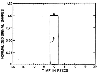
Figure 1.1 Ultrafast opto-electronic switching structure consist- consist-ing of gapped microstrip line evaporated on semi-insulatconsist-ing GaAs

The distorted output pulse is the sharp peak that is barely visible at the leading edge of the input pulse. First is that extreme distortion can occur depending on the initial shape of the wrist.

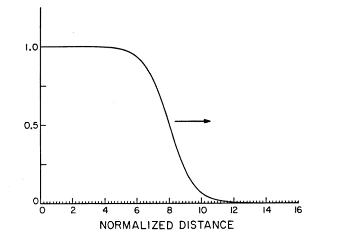
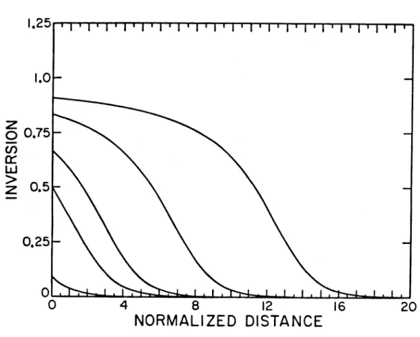
Figs 2.4-7 show the effects on four different pulse shapes for two di.tierent values of G 0 , where the output pulse shapes ~out(t) have been normalized so their peak height is the same as the input peak height of q(t)

NORMALIZED DISTANCE

However, for large intensities the absorption is very non-linear and the bleaching wave propagates well into the material before it loses its "punch". In a real situation, the initial behavior for a high intensity wave (We > 1) will be the bleaching wave result Eq.

Fig. 2.9 shows the steady state solutions Eq. 2.91 with the z axis in units of (aabsN)- 1 , and the vertical axis showing N2 normalized to its maximum (rpe = oc) value of aabs;(aem + aabs)

Appendix A2a

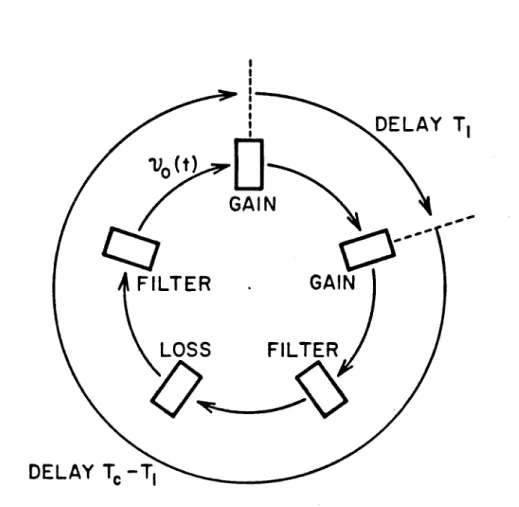
To compare with the results of the previous chapter. which is easily integrated to yield. 3.22 is the time-varying lagged gain defined by Eq. To show the versatility of Eq. 3.20, we next use it as the basis of a brief discussion of the physics of synchronously mode-locked dye lasers.

Figure 3.1 Collinear pump 9'io(t) and signal 9'2o(t) waveforms simultaneously incident on an amplifying/absorbing medium extending from z = 0 to z = L

TIME

DELAY T 1

GAIN " "

FILTER GAIN

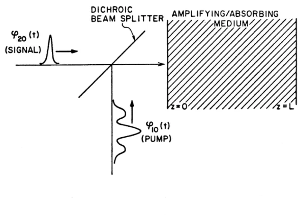
This is the basis of the gate power of a saturable absorber and is exploited in the experimental amplifier system that will be described in detail in Chapter 5. amplifier system.

Figure 3.4 Gain clipping from pump longitudinally bleaching through an amplifier cell with finite 7'

OF PHOTONS/CM 2 INPUT

Dynamical Gain Calculations-with Triplet Losses

Here (3 = -lnR lnG~ where R0 is the initial or leading edge loss factor due to triplet. For the pumping process it is sufficient to use the 9/5 "modified" result as mentioned in the last paragraph. Recording of the population structure in the triplet state can also be included in a simple way, and this is explained in appendix A4d.

The main effect of triplet state population is to increase the signal pulse propagation losses. 2.1 we see that the population of the triplet state begins to accumulate by crossing over between systems as soon as the upper singlet state is first populated. This results in an increase in losses at later times due to the absorption of the triplet state population at the upper triplet level.

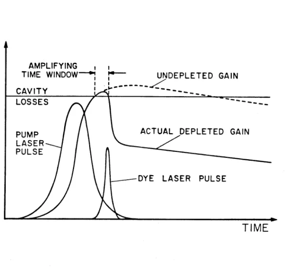
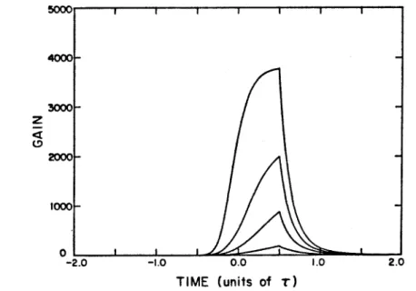
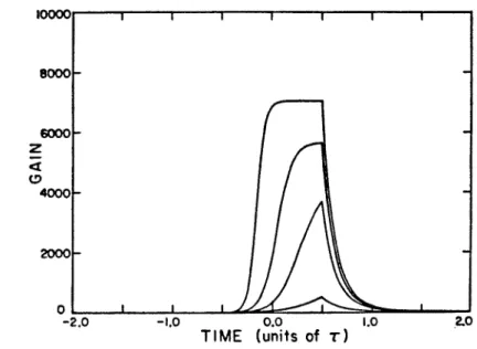
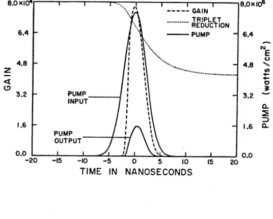
In order to reduce the sensitivity of the gain to the relative timing of the pump and signal pulses, it is desirable to achieve a steady state, which itself requires energy dissipation after a certain point in time. The curves show the input pump pulse, the output pump pulse at the end of a hypothetical amplifier cell, the triplet state gain reduction factor described above, and the small signal gain of the cell (which includes the reduction factor R). The parameters used in these calculations are as follows: The pump pulse was Gaussian with a FWHM of 5 ns, which was also the value taken for the dye lifetime of 7'.

Figure 4.12 Saturation behavior for a hypothetical saturable absorber with G 0 = 10-6 and (Gem+ Gabs)= 4x10- 16 • The dashed curve represents Eq

TIME IN NANOSECONDS

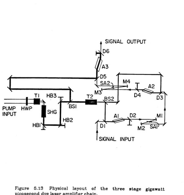
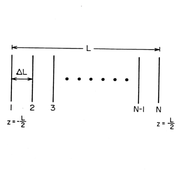
A4b.5 and then evaluate the resulting equation at TJ = L, where L is the length of the amplifier cell. In this chapter, we present the experimental aspects of the gigawatt picosecond laser oscillator and amplifier system. We begin with a brief discussion of the measurement techniques used in this work to study picosecond phenomena in the time domain.

The rise time of the diode was measured with the mode-locked color laser output. These formulas will be essential in the interpretation of the results of the measurements in Chapter 7. The constant K depends on the functional form of the deterministic envelope curve, for which TFWHY is a parameter.

Autocorrelations of the mode-locked dye laser pulses obtained by this method are shown in Figures 5.5 and 5.6; the full scale in both cases is 43.4 psec. 5 corresponds to a better tuning of the oscillator, with an autocorrelation width of B psec, indicating a sech2 pulse width of . The 'real time' aspect of the autocorrelation device described above is essential to the dye laser oscillator adjustments.

Longer pulses are obtained by lengthening the cavity, although due to the excess bandwidth of the cavity, long pulse width operation was almost impossible. Another effect of the finite spatial extent of the beams is the so-called "birefringence" effect.

Figure 4.14 Full dynamic gain calculation, with all parameters identical to those in Fig

EXTRAORDINARY FUNDAMENTAL

FUNDAMENTAL

EXTRAORDINARY SECOND

HARMONIC

Thus, rp can be easily varied by small adjustments of the flashlamps with only small associated changes in the Nd:YAG pulse energy. 8%, while the sub-nanosecond fluctuation in the temporal position of the nodes relative to the Q switch trigger signal was almost negligible. At a fixed point in the counting sequence, one pulse generator is activated to ignite the flash lamp of the Nd:YAG oscillator.

100 nsec with very little jitter, this control is used to determine the relative timing of the pump pulse and the arrival time of the signal pulse at the input side of the amplifier cells. 99.8% of the fundamental separation and beam BS1 sends 80% of the energy down a delay line to the third stage A3, while the remaining 20% is telescoped from T2 to. The path length is adjusted in the table to ensure that the relative arrival times of the signal and the pump beams are the same in all three phases inside.

In the manner described in Chapter 4, this provides good leading edge control to prevent pulse 8 from spreading, but still passes - 75% of the pulse energy. Choosing the laser dye for the oscillator and amplifier requires an accurate knowledge of the variation of the cross-section with wavelength. This is due to the much larger population of the ground state in the CW case and the overlapping of the emission and absorption cross sections; at the maximum emission cross section, the absorption cross section still has a significant value, except for dyes with an exceptional Stokes shift.

Figure 5.13 Physical layout of the three stage gigawatt picosecond dye laser amplifier chain

ANGSTROMS

WAVENUMBERS

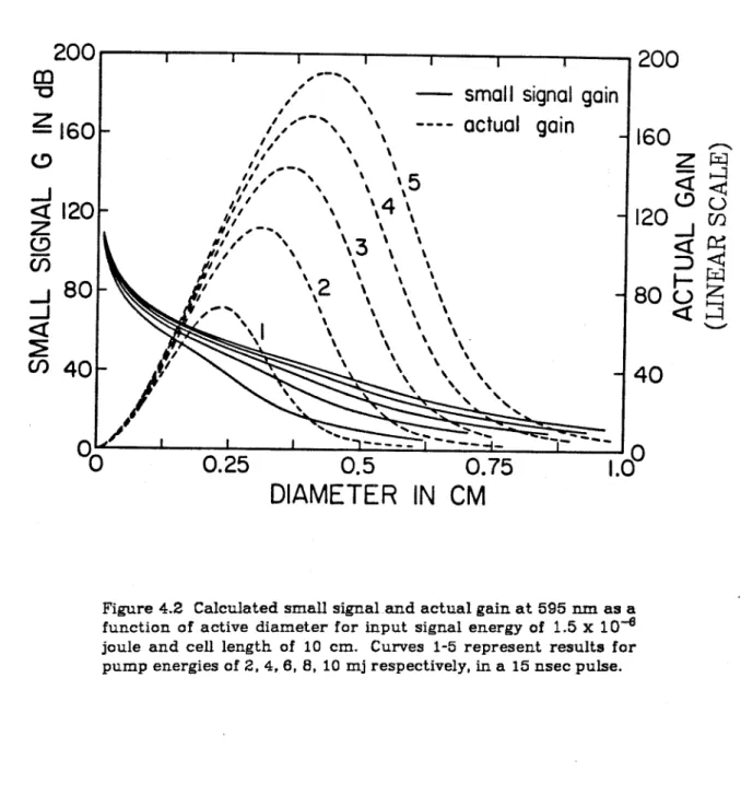
Other workable dyes are Kiton Red or Rhodamine B which are slightly yellower, and for operation in the green or red extremes of the oscillator laser range, Rhodamine 6G or DCM respectively have been successfully used. Matching the desired amplifier spectral range with the peak emission cross section is essential due to ASE depletion. The gain-dependent lifetime Te:ff discussed in Chapter 4 depends on the peak gain G0 occurring near the peak emission cross-section under Q-switched pumping.

It is also necessary for the dye to have a reasonable absorption cross-section at the pump frequency. The output of the amplifier system has energy up to 0.7 mj with no pulse broadening unless the saturable absorbers are intentionally misadjusted by a large amount. Fluctuation in the amplified pulse energy was measured at ::; ± 6% P-P which was actually a little less than the frequency doubled pump laser energy fluctuation at the time of the measurement.

The spatial profile of the pulse is very good at all points throughout the amplifier chain. To observe the dependence of the temporal gain profile on the temporal profile of the pump, the on-axis ASE was monitored with a PIN photodiode. 5.22-24 show the experimentally observed on-shaft ASE along with the pump for three ditherent settings of the rp stage of the ci.adjustable pump discussed in the context of Eq.

10 PSEC

OF PHOTONS/cm 2 INPUT

The essential ingredient of the laser cavity is the optical feedback provided by the end mirrors, and this feature is included in the boundary conditions for Eqs. Here we make no attempt to discuss the coherence properties of the pulsed optical fields of semiconductor lasers. For a general discussion of the gross features of short-pulse evolution, we temporarily introduce the full set of equations Eqs.

A measure of pulse width in time is obtained by dividing the energy in Eq. Also, since the gain in the cavity is modulated on a TRT time scale, the spectral width of the "modes" themselves can become comparable to the space between the modes. The analysis there used the TW rate equations, and therefore we should expect that Eqs.

In the frequency domain this would mean that there is some physical process that 'locks' .. the relative phases of the modes just as in the application of the TW equations to mode locking. Here the physical process was the temporal modulation of the cavity in conjunction with the non-linear gain medium This is exactly the behavior depicted in the output of the Q-switched Nd:YAG output shown in Fig.

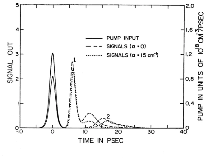
Figure 6.1 Discrete spatial grid used for full T.W. cavity rate equa- equa-tions.

TIME IN PSEC

30% higher for the most accurate equations, but delays and pulse widths were the same within a few percent. the peak power was also the same for both solutions within a few percent. These small differences are probably due to the approximate inclusion of mirror losses in the spatial averaging model using the photon lifetime concept, as well as inherent inaccuracies in the spatial averaging of nonlinear products[3]. To illustrate the effects of round-trip modulation, a mode-locking feature is included by pumping only half the cavity.

For each of the two pumping levels there are a pair of signal curves, one dashed and the other dashed. Results for two different pumping levels are shown labeled 1 and 2. Two sets of curves are shown with each of these to demonstrate the effect of a small additional distributed loss a. .. the expected period TRI'· The spatially asymmetric original noise distribution "rattles back and forth" in the cavity, developing into a short packet with TpuJse < TRI'. The energy localization is probably aided by the unpumped end of the cavity which as serves as a saturable absorber.

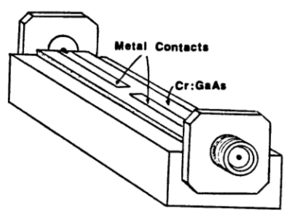
However, an additional factor is that the pulse width is also comparable to 'T"p, because as 'T"p is reduced by a. to increase, the loudness on the pulses is suppressed. The essential feature of this device is that the unpumped central region provides significant loss to the cavity, allowing the laser to be electrically pumped to an initial average gain I'")'o greater than the threshold gain rl'T in would be the absence of the central region losses The pulse width of the dye laser was typically ~ 2 psec as determined by the KDP SHG autocorrelation measurement techniques discussed in Chapter 5.