7 Mid- and high-frequency problems in vehicle noise and vibration refinement – statistical energy analysis. This book provides a review of noise and vibration refinement principles, control methods, and advanced experimental and modeling techniques.
Introduction
This chapter summarizes the objectives and significance of vehicle noise and vibration refinement, defines its scope and illustrates its relationship to the vehicle development process. Some vehicle noise and vibration terms are defined and a brief history of driving and vehicle refinement is presented.
Objectives and signifi cance of vehicle noise and vibration refi nement
Scope of vehicle noise and vibration refi nement
They expect their new purchase to be better equipped, more comfortable, and perform better than the vehicle they just traded in. If the new vehicle is better than the old in every way but lacks refinement, the customer will not be fully satisfied.
The vehicle development process and vehicle noise and vibration refi nement
Mule vehicles are built by modifying the previous vehicle development models in the prototype Alpha where components or system designs are installed. The hybrid simulation is also used to set targets for vehicle development in the 'V' approach.
Vehicle noise and vibration term defi nitions
By performing engineering in advance, the performance targets can be established more accurately, and thus better strategic decisions about vehicle design can be made. In this way, time and expense can be saved later in the lower part of the 'V', as fewer prototype test cycles are required.
History of motoring and vehicle refi nement
In 1876, Emile Berliner, Elisha Gray and Alexander Graham Bell invented the first microphone used as a telephone voice transmitter. The microphone connected to the first articulated telephone transmitter was the liquid transmitter of 1876.
Benchmark analysis together with CAE modeling facilitates vehicle noise and vibration target setting and target cascading. This chapter summarizes the objectives, importance and scope of vehicle noise and vibration target definition and comparison.
Introduction
Objectives and signifi cance of vehicle noise and vibration target setting and benchmarking
The purpose of the benchmarking study is to identify a best-in-class competitor and facilitate the setting of noise and vibration targets for the vehicle's system, subsystems and components. Without this, individual system suppliers would interpret the appropriate level of noise and vibration for themselves.
Scope of vehicle noise and vibration target setting and benchmarking
Excessive noise and vibration caused by one component or subsystem in the intended production vehicle will cause it to fail the design validation test, lead to a large cost increase and time delay for the program, and jeopardize the program targets. The purpose of vehicle noise and vibration target setting is to ensure that the newly developed vehicle has no noise and vibration complaint issues and has superior noise and vibration performance when released on the market.
Benchmarking of vehicle noise and vibration
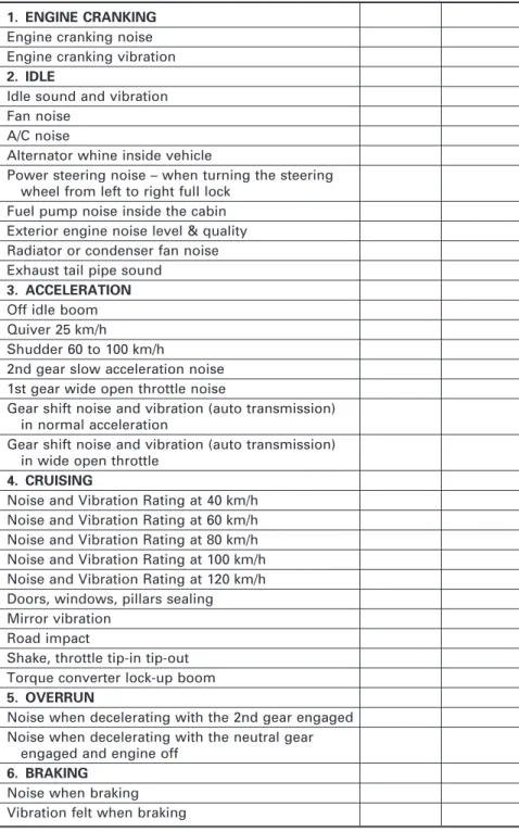
The noise and vibration targets for the whole vehicle system, individual components and subsystems are documented in the overall vehicle specification and system specifications by the brand owner, and compliance with them has become a contractual condition for all suppliers implementing an advanced product quality planning process. In accordance with the vehicle noise and vibration targets, a benchmark study of competitor vehicles shall be conducted for interior and exterior noise and vibration performance, both subjective and objective, of the entire vehicle and of components/subsystems, and of the level and quality of all vehicles operating conditions.
Target setting for vehicle noise and vibration
Transmission Path Analysis (TPA) cascades system-level noise and vibration targets down to subsystem-level targets (Figure 2.5). Noise and vibration measurements will be performed on both the reference and target vehicles under various load conditions.
Summary: This chapter introduces the basic concept of vibration measurement, illustrates the prerequisites for vibration testing and environmental testing, and provides tips for installing vibration objects. The quotation method for vibration levels and the measurement method for complex modulus and damping loss factor are also discussed.
Introduction
Two case studies are provided to illustrate how the principles and methods are applied to solve engineering problems. Keywords: vibration transducers, accelerometers, subjective evaluation, hand detection, proximity sensors, speed sensors, load amplifier, power supplier, Young's modulus, damping loss factor, human vibration limit, vibration isolation, vibration damper.
Hand sensing
Using the human ear for frequency analysis of vehicle noise is more effective when the ear can be connected directly to the vehicle. This is the whole purpose of vibrational instruments – to amplify vibration and display it in a way that we can better understand.
Basic vibration measurements
- Types of vibration transducer
- Selection of appropriate accelerometers
- Charge amplifi ers
- Calibration of accelerometers
- Excitation
They cannot be used on lightweight structures because of the mass loading effect - they change the vibration characteristics of the component whose vibration they are trying to measure. The output impedance of the accelerometer must be matched to the impedance of the reading instrument to accept the signal from the accelerometer.
Vibration response investigation and vibration testing
The force produced by an exciter is mainly limited by the heating effect of the current, i.e. the behavior of the structure is most easily studied with a stroboscopic lamp, activated by the exciter control to follow the excitation frequency, as shown in Fig.
Environmental testing
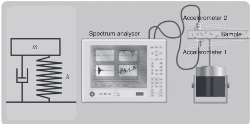
This concept is found, for example, in determining the ability to transmit or damp vibrations, or in the description of vibration modes of a structure at resonances. When calibrating transducers, a comparison is made between the transducer to be calibrated and a reference transducer at a prescribed vibration level.
Mounting the test object
To minimize the weight of the luminaire, it can be constructed from relatively thin plates, supported by brackets. Heavy test objects will cause static deflection of the exciter table, depending on the stiffness of the fixtures.
Measuring the complex elastic modulus
At the resonant frequency ω0, the real part of equation 3.2 becomes zero and the amplitude is determined by the damping mechanism c.
Quoting vibration levels
- Single-value index methods
- Acceleration levels (dB)
- Velocity levels (dB)
- Assessing vibration levels – human response to vibration
ISO 2631 Part Vibration and mechanical shock: Assessment of human exposure to whole body vibration - Part 1: General requirements. Different weightings are given for health, comfort perception, different axes and position of the human subject (standing, sitting and lying down).
Vibration isolation
In many systems of the type shown in Figure 3.17, we are interested in transmitting as little vibration as possible to the substrate. The transmitted force can be written as:. 3.43) Assume that F0= kYeiωt is the amplitude of the actual excitation force.
The vibration absorber
These rises can be controlled to some extent by adding damping, but this will reduce the effectiveness of the absorber at ω22.
Case studies
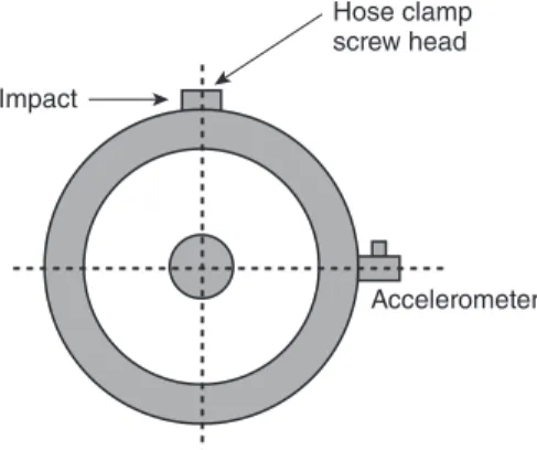
Case study 1
In order to select the best harmonic balancer, candidate parts were supplied to measure the natural frequencies. A pipe clamp was placed on the outer cylindrical surface of the shock absorber ring to provide room for the impact as shown in Fig.
Case study 2: rotational unbalanced masses
The vertical displacement of the two eccentric masses is x + l sin ωt, where x is measured from the equilibrium position. The constant is determined by the mass ratio and the eccentric radius of the unbalanced mass.
Bibliography
Abstract: To develop new vehicle products with well-refined noise performance, vehicle noise measurements and analyzes must be performed to validate design and acoustic refinement. This chapter introduces the physics of sound, sound evaluation methods, basic principles of vehicle noise, human response characteristics to vehicle noise.
Introduction
Key words: wavelength, frequency, amplitude, speed of sound, free string field, diffuse field, condenser microphone, sound pressure level, sound in air, sound transmitted by structure, time and frequency weights, rate of decibel, environmental noise, calibration, octave band frequency analysis, order tracking analysis, waterfall contour spectrum, artificial head technology, psychoacoustics.
Sound fundamentals
- Sound evaluation
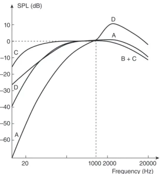
- Human hearing: frequency versus sound pressure level
- Decibel scales
- Decibel arithmetic
Sound levels are generally described in terms of the sound power (W) output of noise sources and the sound pressure (Pa) amplitude at a given location. According to this scale, everyday noise environments fall in the sound pressure level range of 0–120dB.
Vehicle noise
Direct sound-generation mechanics: airborne sound
The combination of two identical sound levels gives a sum which is 3dB greater than the individual levels. Combining one sound level with another that is 10dB smaller in magnitude produces a sum that is negligibly greater than the highest sound level.
Indirect sound-generating mechanism
Measuring microphones
Condenser microphones
The response of the microphone under these conditions is known as the free-field response. The response of the microphone to this artificially higher pressure is the pressure response.
Measuring amplifi ers
Fast – with an exponential time constant of 125 ms which roughly corresponds to the integration time of the ear. Slow – with an exponential time constant of 1 second, so that the average level can be estimated by the ear with greater precision.
Calibration
If the microphone picks up the 94dB sound at 1000Hz from the Type 1 calibrator and shows it as 94dB at the end of the signal chain, it means that the microphone channel passes the calibration. Many people also confirm the calibration at the end of the measurement session.
Background noise
An acoustic calibrator - a small cylindrical device that fits over the microphone capsule and produces a reference sound pressure level at a specified frequency (typically 94dB at 1000Hz; accuracy level is typically ±0.2dB for a Type 1 calibrator) . It is routine to calibrate the signal chain at the beginning of each measurement session.
Recording sound
The sampling rate limit for each digital channel will be the upper limit of the frequency response range divided by the number of channels. High-pass and low-pass filters are set to the correct frequency range to improve the signal-to-noise ratio.
Analysis and presentation of noise data
Single-value indices: pressure–time history
Record levels are carefully set to avoid overloads (a recording level of a recording medium must be chosen to match the dynamic range of the sound).
Frequency-dependent index methods
One of the most commonly used outputs of a constant bandwidth spectrum analyzer is the power spectral density (psd). For each rotation, half of the cylinders have combustion pulses; therefore, half the number of cylinders is the combustion order of the engine.
Artifi cial head technology and psychoacoustics
Only after taking into account the acoustic filter characteristics of the head and ears, accurate and unaltered auditory recordings become possible. Tonality is a measure of the proportion of individual tones or several tone components in a noise.
Bibliography
Abstract: Based on definitions of a linear system, random data and process, the statistical properties of random data, correlation analysis, spectral analysis, the Fourier transform, the impulse response function and the frequency response function are introduced. The relationship between the correlation function and the power density spectrum function, between the impulse response function and the frequency response function, and between the Fourier spectrum function and the power spectrum function is.
Random data and process
- Defi nition of terms
- Time-averaging and expected value
- Mean square value
- Variance and standard deviation
- Probability distribution
- Gaussian and Rayleigh distributions
Stationary random data are defined as data whose ensemble mean statistical properties are invariant with time. Non-stationary random data is defined as data whose ensemble mean statistical properties change with time.
Correlation analysis
Autocorrelation
R(τ) = R(−τ) is symmetric about the origin τ and the vertical axis, which is an even function of τ, as shown in Figure 2.
Cross-correlation
Fourier series
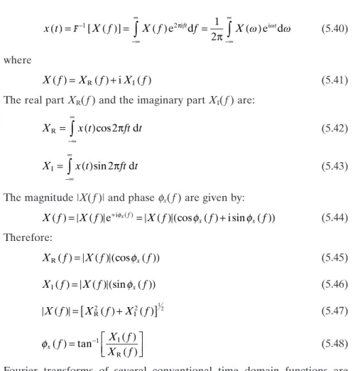
Fourier transforms
The magnitude |X(f)| and phase φx(f) is given by:. 5.48) Fourier transforms of various conventional time domain functions are shown in Table 5.1.
Digital FFT analysis
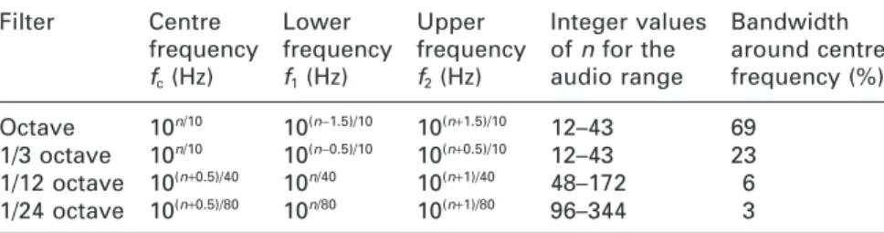
From the average results of the FFT spectrum, the constant-percentage bandwidth filters defined in Table 4.5 and Equation 4.13 in Chapter 4 can be used to calculate the constant-percentage bandwidth spectrum as shown in Table IV (between pages 114 and 115). If a signal process is a non-stationary or transition process, a 3-D spectrum map of the FFT versus time will need to be used to represent the measured spectrum in both the time and frequency domains.
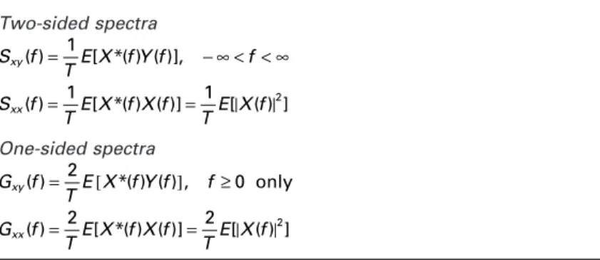
Spectral density analysis
The spectral density functions Sxx(f) and Syy(f) are positive real even functions of f; the cross-spectral is a complex valued function of f. The coherence function of equation 5.59 is a causal relationship unless one has other physical grounds for knowing that an input x(t) produces an output y(t).
Relationship between correlation functions and spectral density functions
Linear systems
Weighting functions
For any linear system, random input data with a theoretical Gaussian probability density function describing its amplitude properties will produce random output data that will also have a theoretical Gaussian probability density function. For a nonlinear system, if the random input is a Gaussian process, the random output is a non-Gaussian process.
Relationship between complex frequency response and impulsive response
Frequency response functions
The inverse Fourier transform relation of Equation 5.97 gives: 5.107) The frequency response function is widely used in the measurement and analysis of vehicle noise and vibration to determine natural frequency.
Bibliography
5.107) The frequency response function has been widely applied in the measurement and analysis of vehicle noise and vibration to determine the natural frequency. Abstract: Structural and acoustic resonances can amplify the excitation acting on an operating tool to levels that significantly degrade noise and vibration performance.
Introduction
Modal analysis is a mathematical tool that allows engineers to determine characteristic values that describe the resonances and then build an analytical model based on this information. With advances in test equipment performance and computing capabilities, modal analysis has become a standard tool in vehicle noise, vibration and harshness (NVH) development throughout the industry.
Application of modal analysis in vehicle development
Spatial, modal and response model
Near a dominant resonance, ODS can look very much like an animation of modal analysis eigenvectors, and indeed, as shown in Fig. Modal analysis uses structural and/or acoustic response data derived through a test with artificial excitation or a computer model of the object's mass.
Application to vehicle NVH development
Each mode of the structure is characterized by its own frequency, modal damping value, and mode shape vectors. Often during vehicle development there is no interest in using a modal model to perform calculations.
Theory of modal analysis
- The physical model
- Forced harmonic vibration
- Multiple degree of freedom systems and modal properties
- Properties of the eigenvalues
The mode shape vectors are scaled arbitrarily; thus the amplitude of the resulting mode shape is not unique and fixed. With the knowledge of the modal frequencies we can now determine the ratio of the displacement vectors x.
Methods for performing modal analysis
- Test-based modal analysis
- Test object setup
- Pre-investigations and data acquisition
- Data analysis
- Predictive modal analysis
After the definition of the response geometry, the test object is set up in the laboratory. Before starting the modal analysis of the measured transfer function data, some health checks should be performed.
Limitations and trends
Modal analysis methods have therefore been developed that allow the simultaneous measurement and analysis of acoustic and structural transfer functions (Wyckaert et al., 1996). For an OMA the test object is investigated under normal operating conditions and only the system responses are measured.
In classical experimental modal analysis, the test object is built up in a lab and artificially excited. Heylen W, Lammens S and Sas P (1997), Modal Analysis Theory and Testing, International Seminar on Modal Analysis, KU Leuven, Belgium.
Introduction
Application procedures of the SEA approach are presented and the most important SEA assumptions are highlighted. Due to the reduced number of degrees of freedom of the models, the SEA calculations are usually very fast (from a few minutes to a few hours), enabling a fast analysis process in the design phase.
Modal approach
Modal resonators and their distribution
The distance from the origin to that point will determine the value of the resonance frequency of the mode ωn1,n2. Each grid corresponds to an area ΔAk=π2/Ap where Ap= L1L2 is the area of the plate.
Energy sharing between two oscillators
The power flow is directly proportional to the difference in decoupled energy of the resonators. The power flow is proportional to the actual vibrational energy difference of the systems, the constant of proportionality being B.
Energy exchange in multi-degree- of-freedom systems
Assume that the spectral densities of the modal excitations are Fiα(t) =∫piψiαdxi fl at over a limited frequency range Δω and that within this band there are Ni= niΔω modes of each subsystem. The modal energies of the subsystem 1 modes are all equal; that is εα = ε1 = constant and εσ=ε2= constant.
Wave approach to statistical energy analysis (SEA)
Averaging the fields in the ensemble gives the diffuse echo field with the state of maximum entropy. The load on the diffuse echo field is proportional to the energy density and group velocity of the subsystem.
Procedures of the statistical energy analysis approach
Defi ning the system model
Divide the system into appropriately sized physical components and combine the natural modes of each component into groups (subsystems) with similar characteristics.
Evaluating the subsystem parameters
Evaluating the response variables
Evaluation of the statistical energy analysis subsystem parameters
- Modal density and group velocity for one-dimensional wave propagation
- Modal density and group velocity for two-dimensional wave propagation
- Coupling loss factor
- Transfer matrices and insert loss of a trim lay-up
- Leaks
- Energy inputs
The force on the junction due to the diffuse incident wavefield (with unit energy density) in the excited subsystem is then found. Loading from diffuse acoustic field excitation can be calculated using the diffuse field reciprocity principle.
Hybrid deterministic and the statistical energy analysis approach
The point force excitation input power used for point/line/area type connections can be calculated from the direct field impedance, which is the same as the calculations performed when calculating the coupling loss factors. The input power due to the excitation of a diffuse sound field is in principle proportional to the radiation efficiency.
Application example
In this way, the coupling effects of the solid structure and the fluid cavity were taken into account in the SEA coupling loss factors. In the frequency range of 0–100Hz, the deterministic method showed modal information in detail; the SEA method provides no modal information and has poor calculation accuracy in this frequency range.
In order to confirm the average SEA energy estimates, a deterministic analysis was performed using a modal expansion in which the effects of solid-structure and fluid-cavity coupling are considered. SEA and hybrid methods tend to overestimate mean response energy levels compared to discrete sample mean/median values from deterministic low- to mid-frequency results.
Introduction
A wide variety of CAE tools and analysis methods are available on the market to simulate certain aspects of sound and vibration refinement. Sound and vibration refinement encompasses many different aspects; therefore, a wide variety of CAE tools and methods are available on the market to simulate certain aspects of sound and vibration refinement through analytical methods.
Basic simulation techniques
- Finite element-based techniques
- Boundary element-based techniques
- Multi-body dynamics
- Tools for system dynamics
- Statistical energy analysis methods
- Computational fl uid dynamics (CFD)
- Transfer path analyses (TPA)
Powertrain FE models for use in vehicle noise and vibration refinement represent the engine (this model is predominantly solids), transmission, and driveshafts. A typical application for noise and vibration refinement is the prior simulation of noise reduction systems.
Frequency or time-domain methods
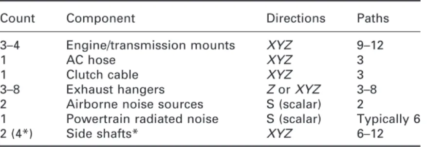
For each TPA, a vehicle is characterized by its "sound paths" rather than its actual geometry. If the latter cannot be predicted with great certainty, they should be based on measured sound sensitivities.
Simulation process
- Virtual series
- Noise and vibration refi nement deliverables for virtual series
- Simulation of design status versus x-functional optimization
- Confi dence in noise and vibration refi nement simulations
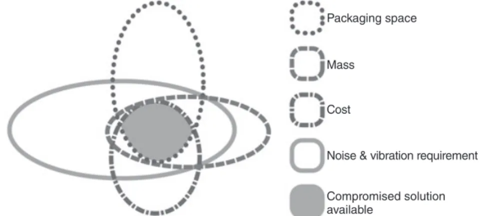
The attributes that offer the most potential conflicts for noise and vibration improvement are vehicle dynamics, durability, weight and cost. Consequently, a 'full analytical score' for improving vehicle noise and vibration is not yet achievable.
Application of virtual reality for vehicle noise and vibration refi nement
Visualization of simulation results
Quality and confidence in CAE simulation results depends on the quality of every single submodel involved. Some vehicle noise and vibration refinement phenomena can be predicted with high confidence by CAE (e.g. powertrain rigid body modes in a vehicle, bending frequencies of a powertrain), while prediction of some other noise and vibration refinement characteristics (clipped body noise transfer functions) cannot be an accuracy of less than say 3dB is not predicted.
Auralization of simulation results
Conclusions
A final note on CAE simulation is that any CAE model that generates errors will definitely give wrong results; CAE simulations without warnings can be correct - nevertheless it is important to understand both the physics and the limitations of each CAE method and model. It is significantly better not to publish questionable CAE results than to share erroneous CAE results that drive the wrong design directions.
Sources of further information and advice
Nevertheless, developers should use simulation techniques for sound and vibration refinement as they are viable contributors to quality vehicles. Summary: This chapter discusses advanced techniques to correctly measure vehicle noise and understand its underlying causes.
Transfer path analysis technique
The difference between the calculated response and the measured response can be used as an indication of the quality of the TPA model. Since the desired response is used as a target for the least-squares optimization, the difference between the measured response and the calculated response can no longer be used as a quality indicator of the TPA model.
Sound intensity technique for source identifi cation