Volume VII No. 1 - April 2023/Page: 25 - 82 https://doi.org/10.36574/jpp.v7i1.366
Article
Indonesia Agricultural Transformation: How Far? Where Would It Go?
Muhammad Abduh1
Corresponding author. Email: [email protected] Submitted: 2022-11-28 | Accepted: 2023-05-08 | Published: 8th May 2023
Abstract
This research examined the inequality that emerges as Indonesia's economy shifts from an agricultural to a non-agricultural sector at the subnational level. These research questions include: (1) How has the agricultural sector in the Indonesian provinces changed over the past two decades? (2) What was the widespread impact of several socioeconomic variables on the transformation of agriculture? (3) How has the agricultural sub-sector responded to the dynamics of these socioeconomic factors over the last decade? The scope of the analysis was the whole province of Indonesia, with time series between 2001-2018. The shift in agriculture at the provincial level was mapped using indicators of poverty and the sector's economic contribution to each province. The logistic regression method was used to see the impact of socioeconomic factors on the agricultural transformation. In contrast, the panel regression was applied to respond to the dynamics of the agricultural sub-sector in terms of socioeconomics in the last ten years. According to the findings of agricultural transformation mapping, there were no changes in the distribution of rural poverty or the agricultural contribution factors between the provinces. Several macroeconomic, social, and infrastructure development factors also significantly contributed to encouraging agricultural transformation and enhancing the added value of the agricultural sector as a whole. It was important to better efficiently utilize the economic potential, which was done by taking production efficiency into account. Furthermore, consumer behaviour and the level of worker productivity had to be considered in attempts to boost economic productivity.
Keywords: provincial disparity; agricultural transformation; agricultural sector development.
1 Regional II Directorate, Ministry of National Development Planning/Bappenas.
1. Introduction
1.1. Background Analysis
The development of Indonesia's agriculture sector over the preceding two decades highlighted some interesting trends (2001–2018). Based on its structure, the agriculture sector's contribution to the economy was decreasing. In 2018, the total contribution of this sector to the national economy was only around 12.23% or Rp. 1,672.35 trillion. It was below the total miscellaneous manufacturing sectors (33.74%) and even the miscellaneous service sectors (45.71%).1 In aggregate, this number seemed good because it denoted a shift in economic structure from the agricultural sector to the non-agricultural sector. However, if we go down to the subnational level, we would find different interpretations in each region.
According to average data from 2011 to 2018, the agriculture sector in Java and Bali contributed 36% of the entire national agricultural sector. Ten years earlier (2000–2010), the share reached 45%, whereas the land area of Java–Bali was only about 10.26% of the total national land area. We will find a contrasting picture when we compare activities in this sector in the Eastern Region of Indonesia (KTI)2, which covers 65% of the total land area of Indonesia, with the Western Region of Indonesia (KBI). KTI’s average annual contribution to the agricultural sector (2011–2018) was only about 25% of its GRDP, while at the same time most of the KTI people still live in rural areas. As an illustration, from 2000 to 2010, the average proportion of the agricultural sector in KTI’s economy was around 68%, although it fell slightly to 64% from 2010 to 2018. Unfortunately, around 80% of the poor people in KTI (out of a total of 6.58 million people) were also trapped in rural areas. Due to the low competitiveness of the agricultural sector in rural areas, the poverty trap may indicate that the transformation process was not inclusive. It happened at the same time that the agriculture sector failed to become the basis of capital accumulation to create sectors that provide greater added value for the economy. Therefore, studying this pattern of change was something interesting to do.
1 Since 2010, BPS has increased the number of economic sector classifications for its GRDP data from nine to seventeen. This modification reflected the adjustment in the base year's calculations from 2000 to 2010. The 2010 base year method was developed using the 2008 National Accounts System as a reference (SNN). Since the SNN is the application of international standards in producing indicators that correspond to economic principles, the calculation of Indonesia's GRDP can be regarded as being in agreement with international standards. Multiple data modifications could be applied across the 17 sectors to either make things simpler or get a particular perspective.
One of them was the three-sector analysis applied by BPS in the publication of employment data.
(see:https://www.bps.go.id/statictable/2021/07/15/2141/rata-rata-pendapatan-bersih-berusaha-sendiri- menurut-provinsi-dan-lapangan-pekerjaan-utama-2021.html). In that report, 17 sectors were simplified into three:
the Agricultural Sector, Manufacturing, and Services. The following sectors were merged to form the service sector:
Trade, Restaurant, and Accommodation Services; Transportation; Warehousing and Communications; Financial Institutions; Real Estate; Rental Business and Company Services; and Community, Social, and Individual Services.
The Manufacturing Sector represents the following sectors: Mining and Quarrying; Processing Industry;
Electricity and Gas Procurement; Water Supply, Waste Management, and Waste & Recycling; Construction.
Meanwhile, the Agricultural sector was independent (it did not consist of a combination of other sectors).
In this paper, the Mining and Quarrying sector was separated from the manufacturing sector category and left to stand alone. So there would be four sectors in the economy of each province. However, the focus of the study in this paper remained on the three sectors of agriculture, manufacturing, and services. The sectors of mining and quarrying were omitted from this analysis to avoid bias. This was because the mining and quarrying reserves in each province vary.
2 Kalimantan, Sulawesi, Nusa Tenggara, Maluku, and Papua.
Stages of development, based on neoclassical theory, start from the agricultural sector and develop into manufacturing sectors and service sectors. Each stage added more value than the sector below it. It was as Lewis (1954) described it. 3 Ranis and Fei (1961) simplified it further. 4 Lewis (1954) said that there were two economic sectors: the traditional sector, which predominated in rural regions, and the agricultural sector. Then there was the modern sector, which was primarily located in urban areas and comprised both manufacturing and services. An economy with the traditional sector as its primary sector arose from underdeveloped conditions. Lewis described rural farmers working with a subsistence ethic, assuming labor was the primary resource in production. It was demonstrated in activities based on basic food needs with a zero marginal production value. It implied that these farmers earn an average wage. Over time, businesses in urban areas (manufacturing and services) began to grow and offer higher wages than the agricultural sector, while also being profit-oriented. Assuming that farmers have thought rationally, when urban sector activities expand and require labor as input, it would be met in abundance by taking it from the agricultural sector. Lewis (1954, in Ranis & Fei (1961)) also described how profitable urban sector activities would increase the amount of capital available for production operations.
The production will then be done on a larger scale in the following cycle, which will enable the absorption of additional rural workers. These workers’ mobility from the traditional sector (agriculture) to the modern sector (urban) was what caused the structure of the economy to shift, from an economy dominated by the agricultural sector to an economy dominated by the modern sector.
Based on Lewis's hypothesis, the various contributions of the agricultural sector at the subnational level of the Indonesian economy in the last two decades have become interesting to study. This diversity could signal economic stagnation rather than a blessing.
This paper contributed to the study of structural transformation by addressing the significance of the agriculture sector to Indonesia's economy (Syirquin, 20085), This study would later be useful in providing additional information in the formulation of well-targeted strategic policies for regional development in Indonesia amidst the shifting economic structure that is currently taking place.
1.2. Context of Indonesia's Agricultural Transformation
The agricultural sector has an important role in the Indonesian economy as a developing country. Indonesia’s economy is very promising, with an annual economic growth rate in the last two decades (2001-2018) of about 5.3%. Compared to other countries economic performance, Indonesia's growth rate (5.37%) was above the average growth of middle-income countries (5.16%), lower-income countries (5.06%), and top middle-income countries (5.21%).6 The agricultural sector contributed roughly 12.23% of the total of 17 sectors in 2018, which was higher than the manufacturing sector's 8.43%7 and the service
3 Lewis, W.A. (1954). Economic Development with Unlimited Supplies of Labour. The Manchester School of Economic and Social, 22: 139-191. https://la.utexas.edu/users/hcleaver/368/368lewistable.pdf
4 Ranis, G. and Fei, J.C.H. (1961), “A Theory of Economic Development,” American Economic Review, Vol. 51, 533-565.
5 Syrquin, M. (2008). Structural change and development. International Handbook of Development Economics, 1:
48-67. https://www.researchgate.net/publication/287237769_Structural_change_and_development
6 According to World Bank data from 2011-2018.
7 Processing industry; Electricity and Gas Procurement; Water Supply, Waste Management, Waste, and Recycling;
Construction.
sector's 4.16%,8 according to data from the Central Statistics Agency (BPS). The agricultural sector represented the majority of employment in rural areas and around 28.79% of all employment nationally, far exceeding the averages of the manufacturing (5.52%) and services sectors (4.36%). Agriculture, on the other hand, played a role in distributing economic benefits in rural areas, where economic activity options were more limited than in urban areas. The agricultural sector's share of Indonesia's GDP continued to decrease as the nation experienced transformation. Despite this, a large percentage of rural residents remained in poverty. Farmers also started looking for informal work outside of agriculture at this time, making them the group of people most vulnerable to economic shocks. In this situation, agriculture still plays a strategic role as a safety net for these informal workers.
Our experiences during the crisis of 1997–1998 showed that this sector became "home" for workers in urban areas (non-agricultural sector) who lost their jobs due to the impact of the crisis in 1998 (Warr, 1998).9
The problem arises when this vulnerability condition overshadows transformed countries with the risk of being trapped in the Middle Income Trap. A 2008 World Bank study found that the choice to subsidize the poor was a very popular choice due to the disparities that occur within developing countries. It had the consequences of limiting fiscal space to sustain transfers large enough to reduce the income gap and continue urban demands for low food prices, as well as reducing public goods for growth and social services in rural areas.10
The development gap between provinces is one of the serious problems in Indonesia.
The unequal conditions make the economic structure vary between provinces. This inequality, according to Rosengard and McPherson, frequently results in measurement bias between the national and sub-national levels. They called it "The Sum Is Greater Than The Parts."11 Referring to the Williamson12 at the provincial level, the inequality rate in Indonesia was quite high. In 2010 the figure was more than half (0.730).13 This figure briefly decreased in 2015 to 0.726 and increased again to 0.747 in 2019. The COVID-19 pandemic slowed the economic growth in various regions, thereby slightly lowering the index to 0.740 in 2020. DKI Jakarta played the biggest role in increasing the Williamson index score compared to other provinces. This index simulation, without taking DKI into account, makes the index value only 0.521 in 2010. The value fell in 2015 to 0.457, then again in 2019 and 2020 to 0.407 and 0.404, respectively. It means that DKI's GRDP per capita left other provinces far behind.
8 Trade, Restaurant, and Accommodation Services; Transportation; Warehousing and Communication; Financial institutions; Real Estate; Rental Business and Company Services; and Community, Social, and Individual Services.
9 Peter, G. Warr. (2001). Crisis, Poverty and Agriculture in Indonesia. Economic and Finance in Indonesia, Faculty of Economics and Business, University of Indonesia, 49, 197-228.
10 World Bank (2008), World Development Report 2008: Agriculture for Development, DOI: 10.1596/978-0-8213- 7233-3
11 Rosengard, Jay K., and Malcolm F. McPherson. The Sum Is Greater Than The Parts: Doubling Shared Prosperity in Indonesia Through Local and Global Integration. Gramedia Pustaka Utama, 2013.
12 Aghion, P., & Williamson, J. (1999). Growth, Inequality, and Globalization: Theory, History, and Policy (Raffaele Mattioli Lectures). Cambridge: Cambridge University Press. doi:10.1017/CBO9780511599064
13 In this paper, the CV calculation uses the formula:
The structural transformation strategy is already incorporated in Indonesia's Long- Term Development Plan (PJP) for the period 2005–2025. The document emphasized increasing the added value of primary sector activities, particularly mining and agriculture, as part of the industrialization process approach.14 This strategy also encouraged the economy to increase its competitiveness in the global market, which was pursued by increasing productivity and innovation through the sustained development of human resource capabilities, the creation of technological mastery and application, as well as support for economic stability and the provision of physical and economic infrastructure.15 In addition, enhancing forward and backward linkages in the value chain between sectors was one strategy to boost the economy's added value. The agricultural sector, as a primary sector, had a strategic role in supporting other related sectors. Meanwhile, the strategy to increase global competitiveness was implemented by improving human resource capabilities, creating mastery and application of technology, supporting economic stability, and providing physical and economic infrastructure.
1.3. Research Problems, Research Objectives, and Research Questions
The Middle Income Trap is a big issue in Indonesia's economic transformation. This trap makes a country fail to enter the category of developed countries because the speed of growth is not enough to deliver an economy at a certain level of income that is beneficial for the welfare of its people and economic productivity.16 To address this issue and foster more inclusive economic growth, closing the economic gap between the provinces was prioritized.17 In this context, the agricultural sector could be regarded as a barometer of how far the transformation has come and where it is headed. This paper tried to see the pattern of shifting in the agricultural sector by taking into account the dynamics of socioeconomic indicators at the provincial level. This study also examined the interaction between the agricultural sector and the poverty rate in rural areas. The following questions were addressed in this paper:
1) How has the development of agricultural transformation across provinces in Indonesia evolved over the last two decades?
2) What is the impact of various socioeconomic indicators on this transformation?
3) How has the agricultural sub-sector responded to the dynamics of these socioeconomic factors over the last ten years?
14 National Development Planning Agency, Vision and Long-Term Development Direction (PJP) 2005 – 2025, Ministry of National Development Planning/Bappenas, Jakarta, 2007 – page 32 (see point 6).
15 Ibid (see point 3).
16 Glawe, L., Wagner, H. The Middle-Income Trap: Definitions, Theories, and Countries Concerned –A Literature Survey. Comp Econ Stud 58, 507-538 (2016). https://doi.org/10.1057/s41294-016-0014-0
17 See WDR 2008, Briones & Felipe (2013), Kyunghoon et al (2018), dan Dartanto et al (2017).
2. Literature Review
2.1. Theories of Agricultural Transformation
Discussions on structural transformation have lasted for a long time, and there was no one mutually agreed definition of this (Syrquin, 2008). Therefore it was necessary to put the term “transformation” in this paper, and why not use the term “change”? It made the terminology clear, consistent, and easier to read. Some publications have highlighted that
"structural transformation" has a broader definition than "structural change," notably Syrquin (2008)18 and Rahardja & Manurung (2008).19 Here, "structural change" was described as a persistent change in the composition of economic aggregates over the long term, while "structural transformation" was defined as a structural change accompanied by the dynamics of economic development.20 Measures of "structural change" were often associated with quantitative indicators like economic growth,21 whereas "structural transformation" was a qualitative indicator22 that was frequently associated with economic development activities like urbanization, demographic change, and the distribution of household income,23 including poverty. So, looking at these explanations, this paper chose the term "agricultural transformation" to figure out the structural change that occurs in development from the perspective of the agricultural sector.
Lewis' (1954) theory is one of the most often adopted concepts of structural transformation. Its simple explanation makes this theory useful in many studies in various countries. Over time, this theory received much criticism. Nafziger (2005),24 for example, criticized the absorption of the urban sector from agricultural subsistence workers in one cycle would increase demand for wages in the next cycle. It was because there were not enough workers in the villages to meet the growing demand for labor. It would ultimately disrupt the absorption mechanism of the urban sector in the future. Lewis also pointed out that the urban sector's absorption effect creates a relative reduction in the quantity of food available because farmers in the remaining villages would be increasingly constrained. As a result, there would be an increase in the cost of food products due to the resulting scarcity.
The process of profits accumulating through wages was eventually eroded due to worker demands for wage increases. Another criticism also came from Sen (2019)25 about the difficulty of applying Lewis's theory to developing/low-income countries. The findings showed a tendency for urban workers to move from the agricultural sector directly to the service sector. In this case, the service sector primarily had lower yields than the
18 Syrquin, M. (2008). Structural change and development. International Handbook of Development Economics, 1:
48-67. https://www.researchgate.net/publication/287237769_Structural_change_and_development
19 Rahardja, P & Manurung, M (2008) Teori Ekonomi Makro: Suatu Pengantar, Ed. 4. Jakarta: Lembaga Penerbit Fakultas Ekonomi Universitas Indonesia – page 318.
20 See Syrquin (2008).
21 See Rahardja & manurung (2008).
22 Ibid – page 318.
23 See Syrquin (2008).
24 Nafziger, E. (2005). Economic Development, Ed. 4. Cambridge: Cambridge University Press.
https://doi.org/10.1017/CBO9780511805615.006
25 Sen, K. (2019). Structural Transformation Around the World: Patterns and Drivers. Asian Development Review, 36:2. https://ssrn.com/abstract=3451537
manufacturing sector, even though there was a trend for the manufacturing sector to decrease in developing nations.
Until now, various ideas and other perspectives have emerged to classify the economic development position of an economy in the context of structural transformation analysis. These ideas were very helpful in simplifying the study of structural
26transformation (Kyunghoon et al, 2018). Lin (2018) 27 described this structural transformation of the economy as a change in the sectors and technologies. This is indicated by the shift in employment patterns from the agricultural sector to the manufacturing and service sectors, which offer higher salaries. In the context of agricultural development, Briones & Felipe (2013) outlined the four stages of an economy's structural transformation.28 (1) First Stage: here, the productivity of labor in the agricultural sector was experiencing rapid growth; (2) Agricultural Surplus Stage: Agricultural surplus, in the early stages, began to be used to finance the non-agricultural sector; (3) Integration Stage: The agricultural sector was connected with various sectors through infrastructure improvements; (4) Since integration was complete, people have also started to leave agriculture and go to more profitable economic sectors. Agriculture also started to deteriorate in this period.
In line with Lewis's theory (1954), several studies and reports use agriculture as a milestone to measure structural transformation. About 15 years ago, the World Bank launched the 2008 World Development Report29 titled "Agriculture for Development."
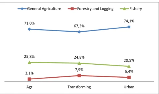
There were three important questions that this report tried to answer. First, what contribution can agriculture make to support the development of an economy? Second, what instruments can be effectively applied to support the idea that agriculture can be used as an engine of development? Furthermore, what kind of agenda would support this? These growing concerns exist because the agricultural sector remains regarded as a vital instrument for promoting development strategies and securing the livelihoods of the poor, particularly in developing countries. The research tried to map every nation in the world according to its individual economic structures in an effort to address the problems. It was done by connecting the poverty indicator to the financial contribution of the agricultural sector. These nations were then divided into three groups using data from 1990 to 2005, including: (1) The agriculture-based countries. This category was characterized by the 32%
contribution of the agricultural sector to its gross domestic product (GDP). Nearly 70% of the poor in this category live in rural areas, which are mainly found in Sub-Saharan countries;
(2) The Transforming Countries. In this group, agriculture was no longer the primary driver of economic expansion. However, the majority of rural areas (up to 82%) remained in pockets of poverty due to the continued dominance of the agricultural sector. Countries that fall into this category were, for example China, India, Morocco, Romania, including Indonesia;
Meanwhile, (3) The Urban Countries were countries where economic activity and pockets of poverty were already dominant in urban areas -with agriculture contributing only about
26 Kyunghoon Kim & Andy Sumner & Arief Anshory Yusuf (2018), Is Structural Transformation-led Economic Growth Immiserising or Inclusive? The Case of Indonesia, May 2018 Working Paper No. 2018/11, Arndt-Corden Department of Economics Crawford School of Public Policy ANU College of Asia and the Pacific.
27 https://bit.ly/3yriyBh
28 Briones, R and Felipe, J (2013). Agriculture and Structural Transformation in Developing Asia: Review and Outlook, No. 363 August 2013; ADB Economics Working Paper Series.
29 World Bank (2008), World Development Report 2008: Agriculture for Development, DOI: 10.1596/978-0-8213- 7233-3
5% of its total growth. The World Bank report30 also listed several possible approaches, including promoting rural agriculture's ability to add value and expanding its non- agricultural economic sector. The agriculture sector continued to serve as the most efficient instrument for household wealth distribution while the transition to secondary and tertiary economic activity continued. A number of alternative policies were implemented, such as creating price incentives, increasing the quality and quantity of investments in public goods, enhancing the quality of the commodity markets, expanding access to financial services, lowering business risk, enhancing the performance of farmer and producer organizations, boosting innovation based on science and technology, and implementing sustainable agricultural practices that improved the environment.
Important roles of agriculture have been an interesting discussion in various scientific works. Johan (2018) saw agriculture plays roles as an instrument in broadly distributing the economy at the macro level, but at the same time, this sector was also able to distribute income to the community at the micro level.31 While Briones & Felipe (2013) highlight the magnitude of the determination of the agricultural sector in various countries in Asia, both countries that have entered the advanced economic phase (such as Japan; South Korea;
Taipei; and China), countries whose agricultural sector still plays a major role (such as Malaysia, Indonesia, and Thailand), to economies whose agricultural sector had not yet grown to its full potential (Bangladesh, India, Pakistan and the Philippines).32 Yifu Lin (2018)33 said that the agricultural sector plays at least three central roles in economic transformation, including economic growth, ensuring food safety, and improving the nutritional quality of the community. The three responsibilities listed above highlight the urgency of agricultural modernization. This agricultural modernization aims to advance industrialization through increased worker productivity, increased agricultural surpluses for capital accumulation, and increased exports. In addition, this upgrade would make food affordable in terms of quantity (lower pricing) and quality (fulfilment of nutritional standards). In addition to changing people's purchasing habits for secondary and tertiary items, modernization also increased people's incomes which would also aid in the community's structural transformation process.
2.2. Transformation in Indonesia: An Analytical Framework
There have been numerous studies done on structural transformation in Indonesia.
Kyunghoon et al (2018)34 examined the relationship between structural transformation and growth inclusiveness in Indonesia. This paper reviewed many aspects of structural transformation in Indonesia, including changes in value-added, trade, employment, productivity, formal employment, and opportunities for low-educated workers in various economic sectors (Kyunghoon et al. 2018). This study was conducted amid the declining
30 World Bank (2008), World Development Report 2008: Agriculture for Development, DOI: 10.1596/978-0-8213- 7233-3, 10
31 Swinnen, Johan (2018). The Political Economy of Agriculture and Food Policies, Palgrave Macmillan, 1 New York Plaza, New York, NY 10004, U.S.A. ISBN 978-1-137-50102-8. https://doi.org/10.1057/978-1-137-50102-8
32 Briones, R & Felipe, J (2013). Agriculture and Structural Transformation in Developing Asia: Review and Outlook, No. 363 August 2013; ADB Economics Working Paper Series.
33 https://bit.ly/3yriyBh
34 Kyunghoon Kim & Andy Sumner & Arief Anshory Yusuf (2018), Is Structural Transformation-led Economic Growth Immiserising or Inclusive? The Case of Indonesia, May 2018 Working Paper No. 2018/11, Arndt-Corden Department of Economics Crawford School of Public Policy ANU College of Asia and the Pacific
manufacturing sector as a growth driver and replaced by the service sector after the Asian financial crisis. It also affected the decline in productivity and absorption level of employment. The added value of manufacturing remains higher than the value added of the service sector in the last two decades. Various characteristics of the economy at the subnational level in Indonesia made the path to structural transformation more complex.
Dartanto et al35 (2017) linked the structural transformation with the phenomenon of income inequality in society. The results of this study supported those of earlier studies conducted in emerging nations that indicated Indonesia transitioned from the agriculture to the service sectors without first passing through the Manufacturing sector. The results of this study using the Theil L decomposition index, both static and dynamic, show that (i) the root of the increase in inequality in Indonesia was pure (unexplained effect); (ii) mobility of the population from the agricultural sector to the manufacturing and service sectors, from rural to urban areas, and from the informal to the formal sector was a secondary contributor in increasing inequality that occurred; (iii) Increasing levels of education have also contributed in increasing inequality in the last two decades; (iv) However, this inequality had eased slightly with an increase in the income of the population who, however, work in the agricultural sector, the informal sector, in the village, as well as with the quality of non- formal education.
Regarding Structural Change, Fitrani (2005) tried to see the phenomenon of growth convergence at the district/city level in Indonesia during 1993-2003 using the Solow model.
In this study, the treatment conditions were classified into absolute and conditional conditions. In this model, the factors of infrastructure, education, and population determined the acceleration of convergence. Meanwhile, Andriansyah et al (2021), in their analysis of structural change indices, found that the pattern of structural transformation generally moves from the agricultural sector to the service sector. In addition, it also found that resource-rich areas and negative Extraordinary Events (KLB) impact the slowness of a region's transformation. This study also discovered that the provinces in Sulawesi experienced the most rapid transformation when compared to others. If this transformation was accompanied by sector-specific growth, it had an impact on long-term regional growth.
3. Data and Method 3.1. Data Sources
Data for this research was obtained from the Central Statistics Agency (BPS) and INDO-DAPOER from the World Bank. The scope of this study was the Indonesian economy at the provincial level. These analyses were classified into descriptive and inferential analyses based on the time sequence. The inferential analysis was performed from 2000–2018, while the descriptive analysis was performed from 2000–2020.36 This inferential analysis was limited until 2018 to rule out the impact of the COVID-19 pandemic, which could interfere
35 Dartanto, T., E. Z. W. Yuan, and Y. Sofiyandi. 2017. Two Decades of Structural Transformation and Dynamics of Income Equality in Indonesia. ADBI Working Paper 783. Tokyo: Asian Development Bank Institute. Available:
https://www.adb.org/publications/twodecades-structural-transformation-and-dynamics-income-equality- indonesia
36 The input data in the model includes data in the range of 2002-2018. The 2000 and 2001 data used include the variables converted into lag-1 (lexpnf_rur_pct, lexpnf_urb_pct, limpor2gdrp, lekspor2gdrp, llnicor) and lag-2 (ldak_pct) data.
with the calculations. The North Kalimantan and DKI Jakarta were excluded from the study as they employed panel data to maintain a well-balanced set of data.
In some cases, BPS and INDO-DAPOER had the same indicators but different figures/values. In these cases, the BPS data was prioritized over the INDO-DAPOER data.
However, in several cases, INDO-DAPOER data had a longer series than BPS data. In this case, the growth pattern of INDO-DAPOER data was calibrated with indicators from BPS.
An example of this was the generation of Gross Regional Domestic Product (GDPR) data.
3.2. Technical Definition of Agricultural Transformation
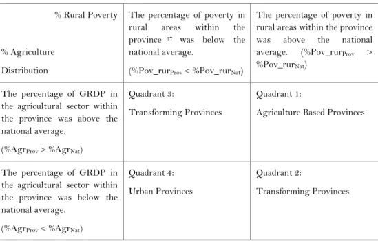
It was necessary to decide on the technical definition of agricultural transformation that would be used in this research to respond to the first question, which was related to the development pattern of the agricultural sector in Indonesia over the past 20 years that occurred in the provinces of Indonesia. The technical definition was modified slightly from the World Development Report 2008's mapping of countries based on how important agriculture was to their development. The mapping was as follows:
Table 1.Technical Definition of Agricultural Transformation
% Rural Poverty
% Agriculture Distribution
The percentage of poverty in rural areas within the province 37 was below the national average.
(%Pov_rurProv < %Pov_rurNat)
The percentage of poverty in rural areas within the province was above the national average. (%Pov_rurProv >
%Pov_rurNat) The percentage of GRDP in
the agricultural sector within the province was above the national average.
(%AgrProv > %AgrNat)
Quadrant 3:
Transforming Provinces
Quadrant 1:
Agriculture Based Provinces
The percentage of GRDP in the agricultural sector within the province was below the national average.
(%AgrProv < %AgrNat)
Quadrant 4:
Urban Provinces
Quadrant 2:
Transforming Provinces
Sources: Author’s formulation
The quadrant boundaries (cut-off) of each variable (distribution of the agricultural sector and the percentage of rural poverty) were the average values in the first decade (2002- 2010). These averages were used as a reference (milestone) to see the transformations formed in the next decade.
These quadrants were analyzed in two steps. The first was general analysis.
Provinces were categorized into three groups for this analysis, which included: (a) Provinces
37 Percentage of Rural Poverty = Rural Poor / (Rural Poor + Urban Poor)
based on the agricultural sector, (b) Transforming Provinces, and (c) Urban Provinces. The categories were transitive in the following order:
(c) > (b) > (a) (1) At this stage, Quadrants 2 and 3 were included in category (b)/Transforming Provinces. Therefore, the type of data formed on this agricultural transformation variable was ordinal.
The provinces represented in quadrants (2) and (3) were separated into two models in the following stage to examine the characteristics and interactions of each socioeconomic indicator. It was important to know the dynamics that occurred in the transforming province. So:
(b2) ≠ (b3) (2) 3.3. Model Specification & Variables
It was required to define the specifics of the study method that was used in order to respond to the second research question, which focused on the response of agricultural transformation to socioeconomic indicators. This study was performed using a quantitative methodology. The methodology selected to get the appropriate inferential analysis results was affected by the use of ordinal data on the dependent variable (agricultural transformation). The Ordered Logit model was used to analyze the model for this kind of ordinal data using the cumulative distribution function (CDF). Because this study used panel data, the application of CDF to panel data was as follows:
pij = p(yi = j)
p(aj-1 < yi* <= aj) = F(aj – xi’b-vl) – F(aj-1 – xi’b-vl) (3) This probability function describes when observation i would choose alternative j. In the ordered logit, F was the logistic CDF, with the form F(z) = ez / (1 + ez).
Following these assumptions, the model specifications were described linearly as follows:
yi = Xitb + vi + eit (4) Note that yi was the dependent variable indicating the number of possible outcomes (in this case: a1 = 1 (Agriculture-based Province), a2 = 2 (“Transforming Province”), and a1
= 3 (Urban Province)). Meanwhile, vi was the identification of the panel coefficient, and eit was a logistically distributed error with zero average and variance of π/3 (Stata, 2019).38
We also could use the Multinomial Logit/Probit Model as an alternative model for this study. However, this paper did not choose this model due to efficiency considerations because it required additional efforts to translate the transitive information of the estimation
38 StataCorp (2019), Stata Longitudinal-Data/Panel-Data Reference Manual Release 16, see page 338 (StataCorp.
2019. Stata: Release 16. Statistical Software. College Station, TX: StataCorp LLC.)
results on the independent variables. This variable was denoted by transform_3, representing the agricultural transformation classification variable defined above (see Technical Definition section 2.2). This variable has three ordinal values, denoted by the notations 1 for a rural province, 2 for a province in transition, and 3 for an urban province.
These three stages were the result of justification to prevent enlargement of the assumption parameter (to be more than three), which would risk the models (William, 2019).39 This variable was the dependent variable in the model (yi).
This paper also explored the "transforming provinces" (b) in more detail. These two quadrants (quadrant-2 and quadrant-3) were analyzed using the logit-panel model by making the outcome in binary form. The new dependent variable was labeled transform_2. This variable was a sub-classification of the transform_3 variable for outcome 2 (Transforming Provinces). The outcome of this binary variable follows: 0 was quadrant-2 (high proportion of rural poverty and low distribution of the agricultural sector), and 1 was quadrant-3 (low proportion of rural poverty and distribution of the agricultural sector was still high).
In order to address the third research question, the analysis then explored the effects that socioeconomic variables had on the performance of the agricultural sub-sector over the past ten years. This estimation identified the most important elements that could help or hinder efforts to promote agriculture. This analysis also explored several perspectives on the transformation of agriculture that had occurred in various provinces in Indonesia. Some of these points of view cover dominant variables in each province, such as the economic, social, and infrastructure. The following covariates (X) were incorporated into the model:
● Social
o A variable that showed the percentage of population expenditure per capita per month for these two types of commodities was necessary to determine the level of public consumption based on the food and non-food goods.
However, this paper also compares expenditure between urban and rural households. So there would be four variables that showed the proportion of consumption based on the area of residence of the population and the type of consumption goods.
These variables include:
𝑒𝑥𝑝𝑛𝑓_ ∗ _𝑝𝑐𝑡 =
𝑈𝑟𝑏𝑎𝑛 (𝑜𝑟 𝑟𝑢𝑟𝑎𝑙)𝑛𝑜𝑛𝑓𝑜𝑜𝑑 𝑒𝑥𝑝𝑒𝑛𝑑𝑖𝑡𝑢𝑟𝑒
(𝑈𝑟𝑏𝑎𝑛 𝑓𝑜𝑜𝑑 𝑒𝑥𝑝𝑒𝑛𝑑𝑖𝑡𝑢𝑟𝑒 +𝑅𝑢𝑟𝑎𝑙 𝑓𝑜𝑜𝑑 𝑒𝑥𝑝𝑒𝑛𝑑𝑖𝑡𝑢𝑟𝑒 +𝑈𝑟𝑏𝑎𝑛 𝑛𝑜𝑛𝑓𝑜𝑜𝑑 𝑒𝑥𝑝𝑒𝑛𝑑𝑖𝑡𝑢𝑟𝑒 +𝑅𝑢𝑟𝑎𝑙 𝑓𝑜𝑜𝑑 𝑒𝑥𝑝𝑒𝑛𝑑𝑖𝑡𝑢𝑟𝑒) The variable of public consumption used in this model was lexpnf_urb_pct (Share (%) of non-food expenditure per month for urban households at the lag-1 year); and lexpnf_rur_pct (percentage (%) of non-food expenditure per month for rural households at the lag-1 year).
39 Williams, R. (2019), Ordered Logit Models – Basic & Intermediate Topics, University of Notre Dame, https://www3.nd.edu/~rwilliam/, (Last revised February 9, 2021)
o Urbanization: the proportion of the urban population divided by the total population in the province. This value showed the share of the urban population in a province.
o s4_ipm_01: number of morbidity (illness) of the population of a province in a year, in the natural logarithm form (ln).
o s4_ipm_03: the average number of years of schooling for people over 25 years old, in ln.
● Economy
o limpor2gdrp: proportion of imports to GRDP at lag-1 year.
o lekspor2gdrp: proportion of exports to GRDP at lag-1 year.
o infl_def_krsna2008: growth of GRDP deflator (%).
o manufpercap: the ratio between the GRDP (constant price 2010) of the Miscellaneous Manufacturing sector to the workers in the respective sector.
o jasapercap: the ratio between the GRDP (constant price 2010) of the Miscellaneous Service sector to the workers in the respective sector.
● Infrastructure
o lnicor: Incremental Capital Output Ratio (ICOR) in ln at the lag-1 year.
o dspesisir_pct: percentage of the number of coastal villages from the whole villages in the province.
o ldak_pct: the ratio between Special Allocation Fund (DAK) and the total revenue of APBD, at lag-2 years.
o lspencap_pct: the ratio between Direct Expenditure for Capital Expenditure (BM) and total Expenditure.
Similar to the previous model specifications, Transforming Provinces would be analyzed further using the Logit model (panel). However, previously the Transforming Provinces were separated first between those included in Quadrant 2 (denoted by 0) and Quadrant 3 (1). These two models were technically compiled with the help of STATA 16 software using the ologit & xtologit commands for the first model (Ordered Logit) and xtlogit for the additional models (Logit).
The estimated coefficients in logistical modeling could not be interpreted as the direct magnitude of interactions between the response variables and their covariates. This is because the coefficients have been converted into log-odds form. As a result, these coefficients must first be calibrated into a more practical form. A feature in STATA 16 allows us to do this by converting the log odds into a probability form.
4. Results and Discussion
4.1. Two Decades of Structural Transformation in Indonesia
In the last two decades, there has been a decline in the average contribution of the agricultural sector and the percentage of the rural poor compared to urban areas in all provinces. The average annual percentage of GRDP in the agricultural sector across all provinces was around 22.7% in the early years (2002–2010), but it decreased to 20.1% in the following ten years (2011–2018). Meanwhile, in terms of the total poverty rate, the trend fell from 70.4% to 68.2% per year in the same period.
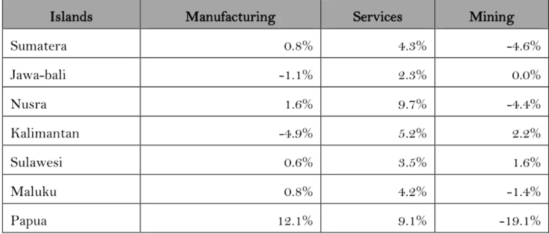
The decline in the contribution of the agricultural sector per province mainly occurred in Eastern Indonesia Areas (KTI)40 by -2.2%. Especially in Nusa Tenggara (-6.9%), Sulawesi Island (-5.7%), and Maluku Island (-3%). The lowest rate of decline occurred in Sumatra Island -0.6% and Java-Bali fell around -1.3%. Growth in the service sector was a major factor in the drastic drop in KTI's agricultural sector (Table 2). The average increase in the service sector in the last decade compared to the previous in all regions reached 5.5%.
In non-Papuan locations, the increase in the manufacturing sector tended to be negative (- 0.4%) on average. Manufacturing saw a surge of about 9.1% in the Papua anomaly, particularly in West Papua. It was related to the commencement of exploration of the Tangguh block for the Liquified Natural Gas (LNG) processing industry. The performance of the regional manufacturing sector and even the economy of West Papua as a whole41 had been significantly impacted by the Tangguh Block, raising concerns about the viability of sustainable economic management in this area.
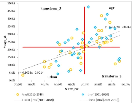
Figure 1. Plot of Percentage of Rural Poverty (%) to Distribution of GRDP in the Agriculture Sector per Province (%)
Sources: BPS & INDO-DAPOER (author’s calculation)
The information above completes the picture of the employment structure in the agricultural sector. Although it was still the main job of the rural workers, the agricultural sector continued to experience a decline in the interest of Indonesian workers from year to year. In the early 2000s, workers in this sector were still the majority (43.78% in 2001), but the trend declined to 28.79% in 2018. Farmers' jobs started to be displaced by jobs in the service sector, particularly informal services (47.97%) and manufacturing jobs (22.06%). The trend of job shifting over the past 20 years had two key characteristics: First, presuming the
40 Includes: Nusa Tenggara, Kalimantan Island, Sulawesi Island, Maluku Island, and Papua Island.
41 Bank Indonesia, 2019. Kajian Ekonomi dan Keuangan Regional Provinsi Papua Barat - Februari 2019. Page 22
non-agricultural sectors could provide a higher added value than the agricultural sectors, and the transition from agriculture to non-agriculture first appeared to be favorable.
However, if we explore deeply, the sectoral shift was not carried out gradually.42 It immediately leaped from the agricultural sector to the service sector. It could be a signal of a structural problem within. If we compared the sector productivity data per worker, the gap between the service sector and its original sector (agriculture) was not very large. The GDP of the service sector was IDR 80.36 million per capita in 2018,43 they were compared to IDR 47.80 million per capita for the agricultural sector. On the other hand, the manufacturing sector outperformed other sectors in the same year, with a productivity per capita of Rp.
165.91 million. Second, the structure of the service sector had a problem of income inequality among its workers. Some types of work in the service sector promise high rewards. However, this sector had a problem with the highest degree of inequality compared to the manufacturing and agricultural sectors. SUSENAS 2018 data showed that the standard deviation between workers' expenditures in the service sector reached Rp. 1,284,423, the manufacturing and agricultural sectors were only Rp 952,356 and Rp 570,843, respectively.
Table 2. The Difference in Average GRDP Contribution of the Non-Agricultural Sector 2011-2018 with 2002-2010
Islands Manufacturing Services Mining
Sumatera 0.8% 4.3% -4.6%
Jawa-bali -1.1% 2.3% 0.0%
Nusra 1.6% 9.7% -4.4%
Kalimantan -4.9% 5.2% 2.2%
Sulawesi 0.6% 3.5% 1.6%
Maluku 0.8% 4.2% -1.4%
Papua 12.1% 9.1% -19.1%
Sources: BPS & INDO-DAPOER (author’s calculation)
In the context of rural economies, the phenomenon of peasant migration to cities in search of jobs could be used to highlight inequality within that service sector.44 Examples are farmers who look for work in the city while waiting for the harvest season or villagers who leave their hometowns because they no longer have land in the village. Because of this, structural adjustments in economic sectors were unable to produce the expected sustainable income growth.
42 Starting from the agricultural sector to manufacturing and then to the service sector.
43 This statistic was calculated by dividing the agricultural sector's GDP in the relevant year by the number of workers within this sector. In the manufacturing and service sectors, the same calculation was applied.
44 Because there were no options.
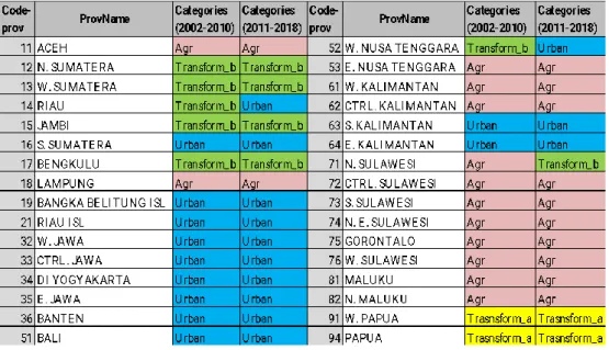
Table 3. Average Category of Agricultural Transformation per Province 2002-2010 and 2011-2018
Sources: BPS & INDO-DAPOER (author’s calculation)
The changes in the agricultural transformation map within Indonesian provinces did not align with the shift in agricultural contribution to the economy and the percentage of rural poverty. According to the criteria of agricultural transformation mentioned above, the number of provinces categorized as agriculture-based provinces (a) in the first decade was 13 (40.6%), while it dropped to 12 (37.5%)45 in the second decade. However, the number of Transforming Provinces (b) had decreased to 7 provinces (21.9%) from 8 (25%) in the previous decade. In the same decade, the urban category (c) increased by two provinces,46 from 11 (34.4%) to 13 (40.6%). Within The Transforming Provinces (b) in Quadrant 2, there was no change in the last two decades (Table 3).
These dynamic situations were associated with several socioeconomic factors. The variables that were used to estimate the logistics model are summarized as follows:
45 Maluku Province moved from the Agriculture-Based (a) category to the Transforming Province category (b).
46 Riau and NTB provinces have shifted from the category of transforming provinces (b) to the category of urban provinces (c).
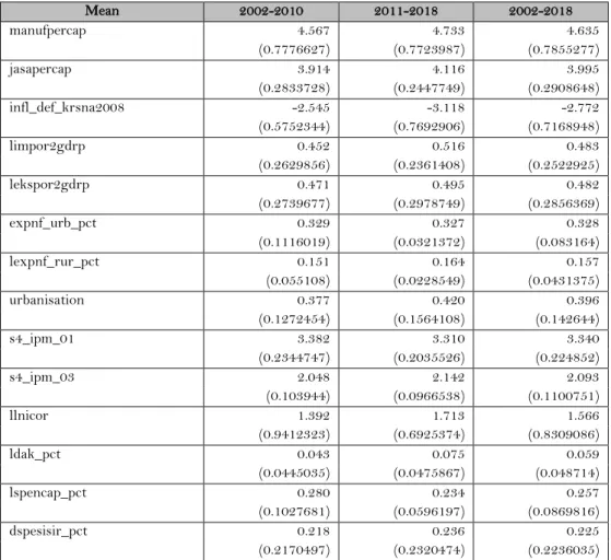
Table 4. The Average of Covariates in Agricultural Transformation Model 2002-201847
Mean 2002-2010 2011-2018 2002-2018
manufpercap 4.567 4.733 4.635
(0.7776627) (0.7723987) (0.7855277)
jasapercap 3.914 4.116 3.995
(0.2833728) (0.2447749) (0.2908648)
infl_def_krsna2008 -2.545 -3.118 -2.772
(0.5752344) (0.7692906) (0.7168948)
limpor2gdrp 0.452 0.516 0.483
(0.2629856) (0.2361408) (0.2522925)
lekspor2gdrp 0.471 0.495 0.482
(0.2739677) (0.2978749) (0.2856369)
expnf_urb_pct 0.329 0.327 0.328
(0.1116019) (0.0321372) (0.083164)
lexpnf_rur_pct 0.151 0.164 0.157
(0.055108) (0.0228549) (0.0431375)
urbanisation 0.377 0.420 0.396
(0.1272454) (0.1564108) (0.142644)
s4_ipm_01 3.382 3.310 3.340
(0.2344747) (0.2035526) (0.224852)
s4_ipm_03 2.048 2.142 2.093
(0.103944) (0.0966538) (0.1100751)
llnicor 1.392 1.713 1.566
(0.9412323) (0.6925374) (0.8309086)
ldak_pct 0.043 0.075 0.059
(0.0445035) (0.0475867) (0.048714)
lspencap_pct 0.280 0.234 0.257
(0.1027681) (0.0596197) (0.0869816)
dspesisir_pct 0.218 0.236 0.225
(0.2170497) (0.2320474) (0.2236035)
Sources: BPS & INDO-DAPOER (author’s calculation)
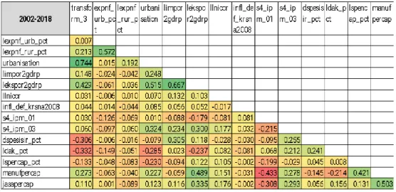
The Pearson test revealed that the covariates with the highest linear correlations to the response variable (transform_3) were urbanization (correlation coefficient=0.744), exports (lekspor2gdrp=0.429), the sum of the Special Allocation Fund (ldak_pct=- 0.322), the number of coastal villages (dspesisir_pct=- 0.306), and manufacturing sector productivity per capita (manufpercap=0.273). On the other hand, there was a low correlation between the average number of school years (s4_ipm_03=0.06), the morbidity rate (s4_ipm_01=0.03), the ICOR (llnicor=0.031), the inflation (infl_def_krsna2008=0.044), and the variable non-food spending of urban households (lexpnf_urb_pct=0.007).
Import (limpor2gdrp) and export (lekspor2gdrp) variables showed the largest aggregate correlation. West Java, Kep. Riau, Bengkulu, Yogyakarta, West Sumatra, South Kalimantan, Gorontalo, Bali, West Papua, and West Kalimantan had the highest correlation value at the province level. At the same time, the lowest occurred in Papua Province: Maluku, South Sumatra, Lampung, Aceh, Jambi, West Nusa Tenggara, East Kalimantan, East Nusa Tenggara, and West Sulawesi. These correlations, however, did not create the specific
47 The number in brackets is the standard deviation.
patterns of the agricultural transformation status of most of the provinces. More than half (56.25 percent, or 18 provinces) of the 32 provinces48 experienced an increase in the average value of the Pearson correlation index between the value of exports and imports in the last decade compared to the previous decade. This growth was regarded as the integration of local business strategies into international trade activities. This strategy was also associated with the flow of urbanization that occurred from time to time, where the correlation index of the urbanization to the export and the import activities was respectively 0.515 and 0.248.
The correlation between urbanization and exports has increased over the past two decades from 0.389 to 0.578. Meanwhile, urbanization with imports also increased from - 0.050 to 0.426. The pattern of non-food consumption of the urban dwellers (lexpnf_urb_pct) to the village (lexpnf_rur_pct) also had a fairly high correlation (0.572). However, this correlation was much changed from the previous decade (0.722) to -0.218 in the last decade.
This fact confirms the assumption that economic progress sometimes contributes to the increasing complexity of urban population consumption patterns. Another relationship that stood out occurred between the GRDP of the Manufacturing sector per capita and the Service sector per capita (0.503). However, this relationship has also declined slightly in the last decade.
Table 5. Pearson Correlation Index for Structural Transformation of Variables Covariate 2002-2018
Sources: BPS & INDO-DAPOER (author’s calculation)
4.2. The Impact of Social Economic Variables in Shaping Agricultural Transformation This paper also examined the relationship between the dependent variable of agricultural transformation, which was ordinal, to a series of socioeconomic variables as the independent variables. Agricultural transformation Variables here were categorical and ordered variables, which assumed the stages of development of an area. This model used the cumulative distribution function (CDF) because it was part of the logistic analysis. Since this
48 North Kalimantan and DKI Jakarta were excluded from the analysis.
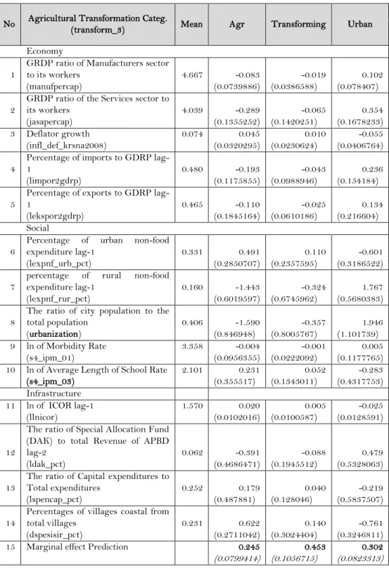
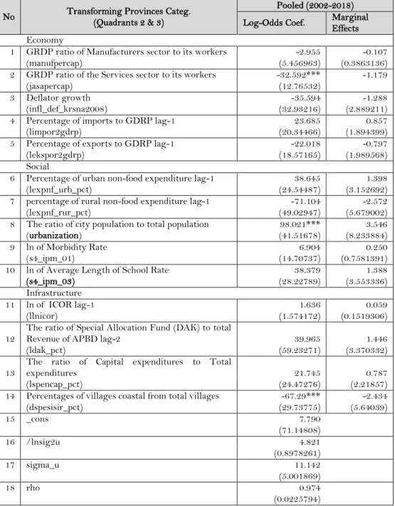
analysis used panel data, the CDF was also calibrated into a panel function.49 Table 6 displays the outcomes of modeling the Agricultural transformation variable and its variables.50 Because the estimated magnitude was in the form of a log-odds ratio (see Table 6), it first had to be calibrated using the cut-off coefficient (/cut1; and/cut2) to obtain the marginal likelihood for each unit change (see Table 7). The "_margins" command feature of STATA 16 was applied for the calibration.
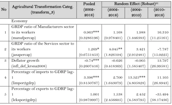
The modeling outcomes shown in table 6 provide several details. Most of the Macroeconomic variables had a significant impact on the transformation of agriculture.
According to Lewis (1954), improving the productivity of the secondary (manufacturing) and tertiary (services) sectors is considered a pull factor for agricultural transformation in each province. In every one million rupiahs per capita, increasing the productivity of the manufacturing sector would increase the likelihood of transformation of provinces based on Agriculture (Agr) into Transforming (Transform) and Urban (Urban) categories by 9.7%, as well as transforming provinces with Transforming category (Transform) into Urban (Urban) by 19.6%. Meanwhile, an increase in the service sector would likely transform agriculture-based provinces into Transforming (Transform) and Urban (Urban) categories by around 28.9% and also encourage the transformation of provinces that were currently Transforming (Transform) into Urban (Urban) provinces by 6.5%.
Table 6. Indonesian Agricultural Transformation Ordered Logit Regression 2002-2018 No Agricultural Transformation Categ.
(transform_3)
Pooled (2002-
2018)
Random Effect (Robust)51 (2002-
2018)
(2002- 2010)
(2010- 2018)
Economy
1
GRDP ratio of Manufacturers sector
to its workers 0.963*** 1.168 1.988 16.310
(manufpercap) (0.3286196) (0.978401) (1.446383) (11.25161) 2
GRDP ratio of the Services sector to
its workers 1.269* 4.045** 3.421 -7.787
(jasapercap) (0.6751453) (1.826104) (2.912481) (15.0225)
3 Deflator growth -0.74*** -0.626 -0.905 13.797
(infl_def_krsna2008) (0.2607416) (0.418369) (1.585407) (26.99581) 4
Percentage of imports to GDRP lag-
1 3.396*** 2.700 13.525*** 11.105
(limpor2gdrp) (0.8150767) (1.643079) (4.805828) (26.8943) 5
Percentage of exports to GDRP lag-
1 1.001 1.538 2.452 -35.494
(lekspor2gdrp) (0.9879997) (2.456605) (4.583795) (38.17436)
49 StataCorp. (2019), Stata Longitudinal-Data/Panel-Data Reference Manual Release 16, see page 338 (StataCorp.
2019. Stata: Release 16. Statistical Software. College Station, TX: StataCorp LLC.)
50 The Pooled Effect and the Random Effect Models were used in the analysis of the Ordered Logit Model discussed above. These two approaches are used to determine the estimators who have had the largest impact on agricultural transformation over the last 20 years. As a result, data from each method can be used simultaneously or interchangeably. In the conventional RE model without robustness, the results of the LR2 significance test comparing the two models suggested that the RE model had lower variance than the standard model (Pooled). (See Table 6, row 22).
51 Robust is a feature in STATA to select the maximum variance estimator to be used in the model based on the score of the equation at a certain level and its covariance matrix (STATA 16 Manuals).
No Agricultural Transformation Categ.
(transform_3)
Pooled (2002-
2018)
Random Effect (Robust)51 (2002-
2018)
(2002- 2010)
(2010- 2018)
Social
6
Percentage of urban non-food
expenditure lag-1 -0.842 -6.872* 13.482 -36.225
(lexpnf_urb_pct) (2.407906) (3.464124) (15.34241) (35.98685) 7
percentage of rural non-food
expenditure lag-1 9.034* 20.203*** 19.760 94.562*
(lexpnf_rur_pct) (4.843767) (4.533783) (19.42558) (55.13867) 8
The ratio of city population to the
total population 25.061*** 22.260** 53.169*** 297.563*
(urbanization) (2.088979) (10.65045) (11.45679) (96.13681)
9 ln of Morbidity Rate 0.716 0.054 2.152 1.913
(s4_ipm_01) (0.7554912) (1.345237) (3.062585) (15.83647) 10 ln of Average Length of School Rate -6.658*** -3.234 -12.011* -90.391 (s4_ipm_03) (1.149855) (4.927691) (6.61164) (106.6864)
Infrastructure
11 ln of ICOR lag-1 -0.163 -0.284** -0.378 -2.504
(llnicor) (0.1355511) (0.123367) (0.265015) (2.478555)
12
The ratio of Special Allocation Fund (DAK) to total Revenue of APBD
lag-2 -0.634 5.480 6.656 23.671
(ldak_pct) (3.508817) (6.204729) (7.37414) (26.52608)
13
The ratio of Capital expenditures to
Total expenditures -2.172 -2.508 6.495 -1.090
(lspencap_pct) (2.361119) (6.674816) (9.988024) (23.73752) 14
Percentages of villages coastal from
total villages -3.569*** -8.707**
-
12.099*** -3.522 (dspesisir_pct) (0.8528296) (3.491913) (4.017916) (9.446938)
15 /cut1 7.695 21.412 35.581 -47.297
(5.128489) (13.74108) (24.51059) (65.41919)
16 /cut2 10.593 26.651 41.532 -9.355
(5.142428) (13.97265) (24.67544) (79.81481)
17 /sigma2_u 16.375 12.066 746.823
(11.8085) (5.287915) (860.094)
18 Log pseudolikelihood52 -219.76834
-
162.17914 -84.85465
- 48.585836 19 Wald chi2(14) 228.13*** 139.38*** 81.1*** 391.78***
20 Number of obs 429 429 238 191
21 Number of groups 32 32 31
22 LR Test in Normal RE Sig. 1% Sig. 1% Sig. 1%
Notes: * significance. 10%; ** 5%; ***1%. The brackets ( ) indicate the standard error Sources: BPS & INDO-DAPOER (author’s calculation)
52 The fit model was only successful up to the 29th iteration due to incomplete iteration processes.
Table 7. Marginal Effect Model Ordered Logit Indonesian Agricultural Transformation Year 2002-2018
No Agricultural Transformation Categ.
(transform_3) Mean Agr Transforming Urban
Economy
1
GRDP ratio of Manufacturers sector
to its workers 4.667 -0.083 -0.019 0.102
(manufpercap) (0.0739886) (0.0386588) (0.078407)
2
GRDP ratio of the Services sector to
its workers 4.039 -0.289 -0.065 0.354
(jasapercap) (0.1355252) (0.1420251) (0.1678233)
3 Deflator growth 0.074 0.045 0.010 -0.055
(infl_def_krsna2008) (0.0320295) (0.0230624) (0.0406764) 4
Percentage of imports to GDRP lag-
1 0.480 -0.193 -0.043 0.236
(limpor2gdrp) (0.1175855) (0.0988946) (0.154184)
5
Percentage of exports to GDRP lag-
1 0.465 -0.110 -0.025 0.134
(lekspor2gdrp) (0.1845164) (0.0610186) (0.216604)
Social
6
Percentage of urban non-food
expenditure lag-1 0.331 0.491 0.110 -0.601
(lexpnf_urb_pct) (0.2850707) (0.2357595) (0.3186522) 7
percentage of rural non-food
expenditure lag-1 0.160 -1.443 -0.324 1.767
(lexpnf_rur_pct) (0.6019597) (0.6745962) (0.5680383) 8
The ratio of city population to the
total population 0.406 -1.590 -0.357 1.946
(urbanization) (0.846948) (0.8005767) (1.101739)
9 ln of Morbidity Rate 3.358 -0.004 -0.001 0.005
(s4_ipm_01) (0.0956355) (0.0222092) (0.1177765)
10 ln of Average Length of School Rate 2.101 0.231 0.052 -0.283
(s4_ipm_03) (0.355517) (0.1343011) (0.4317753)
Infrastructure
11 ln of ICOR lag-1 1.570 0.020 0.005 -0.025
(llnicor) (0.0102016) (0.0100587) (0.0128591)
12
The ratio of Special Allocation Fund (DAK) to total Revenue of APBD
lag-2 0.062 -0.391 -0.088 0.479
(ldak_pct) (0.4686471) (0.1945512) (0.5328063)
13
The ratio of Capital expenditures to
Total expenditures 0.252 0.179 0.040 -0.219
(lspencap_pct) (0.487881) (0.128046) (0.5837507)
14
Percentages of villages coastal from
total villages 0.231 0.622 0.140 -0.761
(dspesisir_pct) (0.2711042) (0.3024404) (0.3246811)
15 Marginal effect Prediction 0.245 0.453 0.302
(0.0799414) (0.1056715) (0.0823313)
Notes: * significance. 10%; ** 5%; ***1%. The brackets ( ) indicate the standard error Sources: BPS & INDO-DAPOER (author’s calculation)
The secondary and tertiary sectors mentioned above require investment support in capital goods and raw materials to enable a proper production process. The national investment rate in 2015 was IDR 3926.2 trillion, or 34.1% of the GRDP, for various capital goods (PMTB) and raw materials (inventory). Imports accounted for 46.32% of that total investment.53 It was relevant to the estimation results above, which show a positive and significant relationship from this import activity. For example, a 1% increase in imports (from GRDP) has the potential to elevate an agriculture-based province to the transforming and urban category by 34.1%. An increase at the same level also has the potential to push the province, which is currently in the transforming category, into the urban category by 37.4%. Unfortunately, the important role of international trade was not accompanied by an improvement in export performance. At the same time, the correlation between these two (imports and exports) was very high compared to the correlation between variables that occurs in other variables. This/it meant that the revenue, which came from exports, was represented by the import capacity at the time. Improving export capacity had to be able to increase domestic income in order to support the agricultural and structural transformation processes.
The secondary and tertiary sectors above, which represent sectors in urban areas, could also be considered a reflection of the potential income and consumption of urban people at the household level. As noted from BPS data, the average annual household consumption in the last decade (2011-2018) represents about 55% of GRDP by expenditure. According to the 2015 BPS data, from a total of Rp 6490 trillion, most of this consumption was spent on food and beverage needs (around 21.65%), followed by transportation and communication needs (23.4%), household furniture needs (7.37%), and the remaining amount (25.08%) being spent on clothing, health care, and other needs. This description also provides an overview of the agricultural sector's role in the consumption sector. The assumption was that the agricultural sector (38.4%) supplied all demands for food and beverages and that non-food consumption products made up the remaining 61.6%.
The estimation results also confirm that non-food consumption had an effect on slowing down the agricultural transformation process. This condition was suspected to be the result of a structural imbalance in the economy, as explained by Baumol's Law of Disease Costs (Chai, 2018). The law explained the interpretation bias in the shifting consumption of manufactured goods and services due to changes in their relative prices due to innovation disruption. This point of view differs from Engel's Law in seeing the shift in consumer preferences, seen through their food and non-food expenditure curves, as income increases.
According to Baumol (1967), quoted by Chai (2018),54 the "disease" began when disparities widened as a result of technological advances in both the manufacturing and service sectors.
Although both are developing, innovation in the manufacturing sector moves faster than in the service sector. This eventually has an impact on the differences in the level of production efficiency of each sector, where the manufacturing sector could perform production costs efficiently and vice versa for the service sector (Chai, 2018). This inequality condition would provide a paradoxical picture of people's consumption activities. It is well known that the
53 2015 Exchange rate: IDR 13795 / US$ obtained from Statista.
54 Andreas Chai (2018), "Household consumption patterns and the sectoral composition of growing economies: A review of the interlinkages," Discussion Papers in Economics economics:201802, Griffith University, Department of Accounting, Finance, and Economics. Page 21