A Millimetre Wave Embroidered Antennas

WLANs and body area networks (BANs) are rapidly advancing as high data rate wireless communication systems using the Ulta Wide Band (UWB) spectrum. In these UWB communication systems, the antenna design plays a key role in signal transmission and reception. However, antenna design in the UWB spectrum is more challenging than a narrowband design. Antenna arrays that form the beam play an important role at these frequencies.

In this work, a new embroidery-type dipole antenna and dipole arrays for body area networks are proposed. The unlicensed 57-64 GHz ultra-wideband spectrum which has a bandwidth of 7 GHz is used for short-range communication [1, 2]. Millimeter waves in this band have high attenuation due to the oxygen and water content present in the atmosphere.

The attenuation for this band is around 12-15 dB/Km and penetration through concrete walls is negligible due to high power loss. The UWB 60GHz band can reach gigabit per second data rates for short-range wireless communications due to the availability of large bandwidth.

Figure 1.1: Millimetre wave band in spectrum [4]

Body Centric Communications

Off-body communications

On-body communications

In-body communications

Wearable Antennas at Millimeter Waves

Previously in this field, many antenna designs for different operating frequencies have been proposed and practically designed. In this work, the proposed antenna designs are easy to fabricate and the designs overcome the above challenges.

Literature and Contributions

The geometry of proposed antenna consists of four semicircular arms to ensure that the length of the antenna is full wavelength, i.e. Length of each arm is λ4 such that the total length is λ. Antenna is symmetrically positioned along YZ axis as shown in Figure 2.1. We can choose off-center supply point and check that current at that point is not equal to zero.

Figure 2.1: Full-wave Dipole Antenna

Current Distribution

Antenna Parameterization

Far-field calculation

Magnetic vector potential

Where µ is permeability, point (X0, Y0, Z0) is the source point and point (X, Y, Z) is the observation point. Each integration in (3.8) is solved using Simpson's 38thrule, and the expressions are given by Ay1= µvIOexp(−jkr).

Magnetic and Electric field calculation

Theoretical and Simulation Results

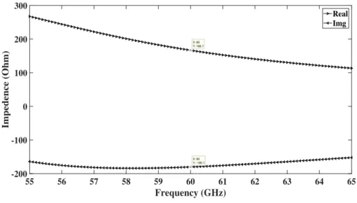
For the antenna resonance, we need to match the input impedance with suitable matching components between the load (antenna) and excitation. We can use single stub matching to match the impedance of the antenna[24] by selecting the appropriate coaxial cable. To make the antenna resonant with a reduced reactive component, we reduced the antenna size as in [18].

Return loss of the proposed antenna shown in Figure 2.6, the antenna resonates at 60 GHz and covers the entire unlicensed ultra wide band from 57 GHz to 64 GHz. From all the graphs, there is a good agreement between the theoretical for all antenna parameters and the simulated results. In Chapter 3, we discussed the multi-turn full-wave dipole antenna with theoretical analysis and HFSS simulation results, the main motivation for this work is to embroider millimeter wave antenna on fabric.

Due to insufficient length, we cannot embroider the 5mm dipole antenna, so we need enough turns for embroidering. We can increase the length of the antenna by increasing the number of turns N (each turn length is λ4). As we increase the length of the antenna, the Far-field radiation pattern is different when we compare it with a double wave dipole antenna.

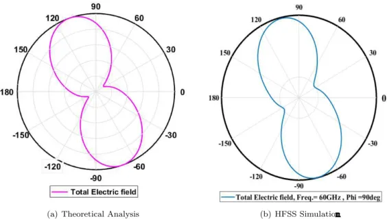
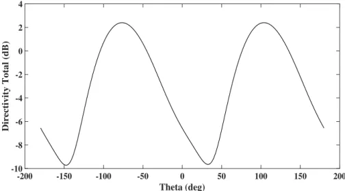
In the straight (linear) dipole antenna, the radiation pattern is the same if we add λ length to half-wave dipole antenna, but in this case for the proposed antenna, it is not the same, so we observed different length radiation patterns. As shown in the figure, the antenna contains N(=6) turns and each turn measurement follows the same as we discussed in the previous chapter full wave dipole antenna. For the linear dipole antenna, the current distribution is sinusoidal [22], for the proposed antenna, we assumed that the current distribution along the antenna is sinusoidal, and it is tangential due to the antenna position on the coordinate axis.

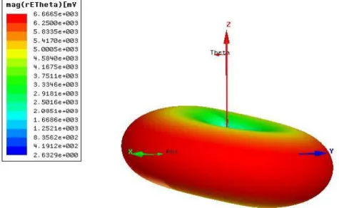
After parametrizing the antenna as described in Chapter 3, we have the tangential flux equations for each turn as shown in the equation below. Looking at Figures 3.2, 4.3, there is a close match between the theoretical and simulated radiation patterns, so we can confirm that the antenna has a sinusoidal current distribution. Figure 4.4 shows the 3D far-field radiation pattern of the 3λ2 antenna, it is different from the previous dipole pattern and we can see the increase in side lobes with the increase in the number of wraps.

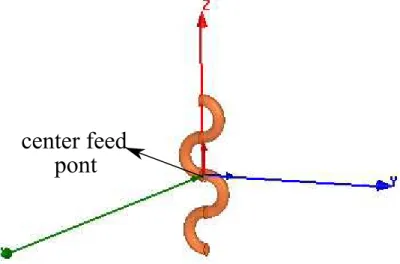
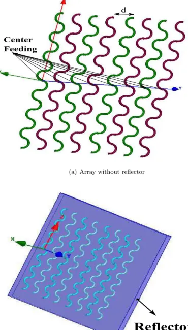
The antenna configuration is shown in Figure 3.3, in that configuration antenna is configured with eight half circles, each half circle arm measurement mentioned in the previous chapter. In this chapter, radiation patterns with different lengths of the embroidery antenna were observed for the dipole radiation pattern.

Figure 2.2: Directivity plot of Proposed Antenna

Conclusion

Introduction

Antenna Array setup

Antenna array with Reflector

Antenna Parameters

• Directivity and Gain
• Radiated Electric field
• Return losses and Mutual coupling
• Antenna feeding and impedance Matching

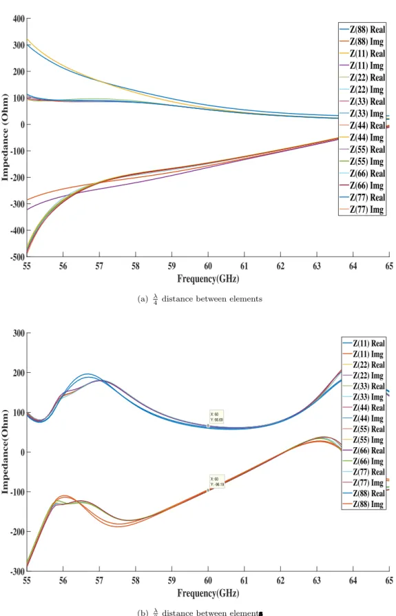
When we have embroidered the array on cloth, we need the radiation along the perpendicular to the antenna axis as shown in Figure 4.4, to ensure that we have chosen theθ= 90◦. Return loss is the important parameter for antenna design, it measures how much power returns to antenna port due to mismatch with the transmission line. When the distance between elements increased to λ2, then the operating bandwidth was reduced as shown in Figure 4.5(b), the occupied bandwidth is GHz.

Mutual coupling is the electromagnetic interaction between the antenna elements in the array, due to mutual coupling current distribution, input impedance and array far-field radiation pattern are effected. As the distance between the antenna elements in the array increases, the mutual coupling decreases [22]. In the proposed array, all antenna elements are center-fed [19, 22], we can choose off-center feed-ed antenna elements to ensure that the current will not be zero at the feed point of the antenna element.

Without reflector With reflector Single antenna element. a) Common E field without reflector (b) Common E field with reflector. Due to the mutual coupling between the elements, there is an influence on the input impedance of both extreme end elements of the antenna, which can be seen in Figure 6(a). As the distance between antenna elements increases, all antenna elements have the same input impedance (approximately) as shown in Figure 6(b).

Figure 4.1: Array Setup

Limitation on number of Antenna Elements and length

Conclusion and Future work

Short-range wireless communications for next-generation networks: UWB, 60 GHz millimeter wave WPAN and ZigBee. Antennas and propagation for body-oriented wireless communications at millimeter wave frequencies: an overview [Wireless Corner]. End-Fire Antenna for BAN at 60 GHz: impact of bending, performance on the body and study of an 'on to off-body' scenario.

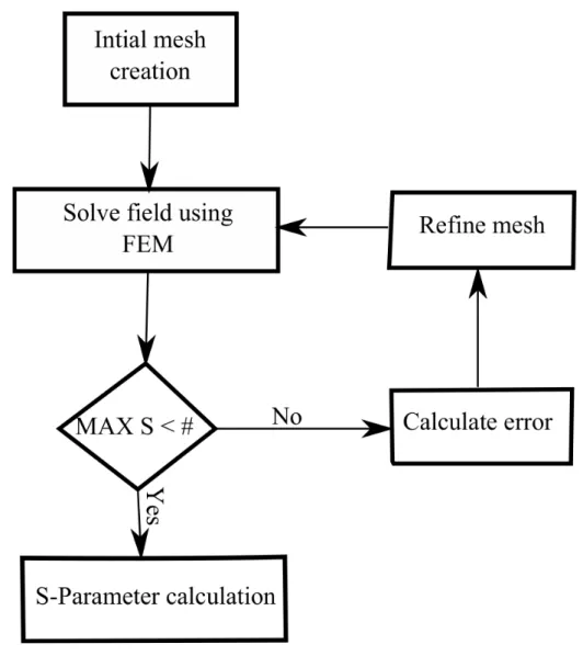
In this procedure the structure we want to simulate is divided into small parts. The iterative process (solution-¿ error analysis-¿ processed mesh) is running until the error converges or the adaptive transitions are satisfied. In this work all simulations completed with 0.02 error convergence and 6 adaptive passes). In this work we only use the radiation limit because the designed antenna model is an open model.

The time required to analyze the given model depends on solution frequency and error convergence rate. In this work, we are mainly focused on the return loss of the antenna and design the antenna so that it creates beam-forming fields in the desired direction.

Figure 4.6: Antenna array Input impedance

Mathematical method used by HFSS

• Adaptive solution

For the fields, a solution is found in each finite element and these solutions are interrelated so that Maxwell's equations are satisfied across inter-element boundaries. So that it finally yields one solution for the whole structure and then found the general S-parameter matrix. Adaptive solution is a mathematical iterative process used by HFSS and it gives a high accuracy solution for a given Electromagnetic field problem.

HFSS calculates the electromagnetic field inside the structure when it is excited at the solution frequency. Based on the current final HFSS solution, find the region of the tetrahedron where the error is large. If we consider that the frequency sweep is the same as above done at each frequency point without mesh refinement.

Figure A.2: Adaptive Pass procedure

Steps followed in HFSS simulation

Materials and Dimensions