It is declared that the work contained in the thesis entitled “Extended Born-Oppenheimer equation and the effect of the external field on the non-adiabatic coupling elements” by Mr. Student of the Department of Chemistry, Indian Institute of Technology Guwahati for the award of Doctor or Philosophy is practiced under my supervision. In the same paper27 they investigate the curl of the non-adiabatic coupling for any realistic description of the electronic wave function.
Adiabatic Representation
The diabatic representation, the transformation from adiabatic to diabatic frames and the relevant curl condition, the Jahn-Teller model and the Longuet-Higgins phase and formulation of EBO equation for two-state system are also discussed. This is the core SE within the adiabatic framework for a given Hilbert/sub-Hilbert space.
Diabatic Representation
The main difficulty here is that the nuclear dynamics is based on a single electronic basis set (calculated atn0). This cannot be an efficient representation because it requires a large electronic basis set that produces a V-matrix with large dimensions and large off-diagonal matrix elements.
Adiabatic-to-Diabatic Transformation
Since A is the (orthogonal) transformation matrix connecting the two frames, we call it the adiabatic to diabatic transformation matrix or as the ADT matrix. In other words, the transformation from an adiabatic frame to a diabatic frame (or vice versa) does not affect the solution of this equation.
The Curl Condition
To conclude this derivation, we claim that the treatment of the Schroedinger equation, whether done in the adiabatic or diabatic representation, gives the same solution. In the following, we need to find the conditions for the mixed differentiation of the Amatrix elements to be order independent.
The nonadiabatic coupling terms and Hellmann - Feynmann theorem
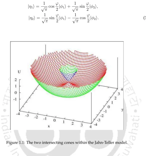
The Jahn-Teller model and Longuet-Higgins’ phase
One way to get rid of the surplus value of the electronic eigenfunctions is by mul-. The fact that the electronic eigenfunctions are modified as presented in Eq.(1.41) has a direct effect on the nonadiabatic coupling terms.
Single-surface Born-Oppenheimer equation for two - state system
In Chapter 2 and Chapter 3, the formulation of Born-Oppenheimer equation for three- and four-state sub-Hilbert space, respectively, was discussed. Bear, Beyond Born-Oppenheimer: Conical Intersections and Electronic nonadiabatic Coupling Terms, Wiley Interscience, Hoboken, N.J., USA, 2006.
Theoretical developments on the Born-Oppenheimer treatment
In order to obtain a meaningful solution to Eq., 2.7), we must ensure that the chosen matrix form has the following characteristics: (a). The BO equation can be written from the matrix equation [Eq. 2.34) by considering the following aspects: (a) Since the matrix.
Summary
We demonstrate1 the explicit forms of the nonadiabatic coupling elements in terms of ADT angles by considering the existence of the ADT state, ∇~A+~τA = 0, for any four-state sub-Hilbert space. Given the explicit forms of the NAC terms for any four-state sub-Hilbert space, we investigate the analytical validity of Curl terms.
The Born-Oppenheimer treatment of a four state sub-Hilbert space
The eigenvalues of NAC matrix
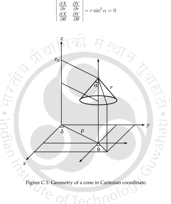
If the origin of the coordinate system coincides with the point of conic intersection, or even if the point(s) of conic intersection is distant from the origin of the coordinate system, the parametric representation for the vector equation of the conic surface (see Appendix C) predicts the validity of the following identities: ∇pθ13. for any pair of nuclear coordinates, namely pandq, at and around the point of conic intersection. When we substitute these identities in Eq. 3.10), the non-adiabatic coupling expression has the following form: and similarly other NAC terms. At this junction we can recall Eq. 3.16) to find the following quantities (A and B) taking into account the NAC elements as presented in Eqs.
Summary
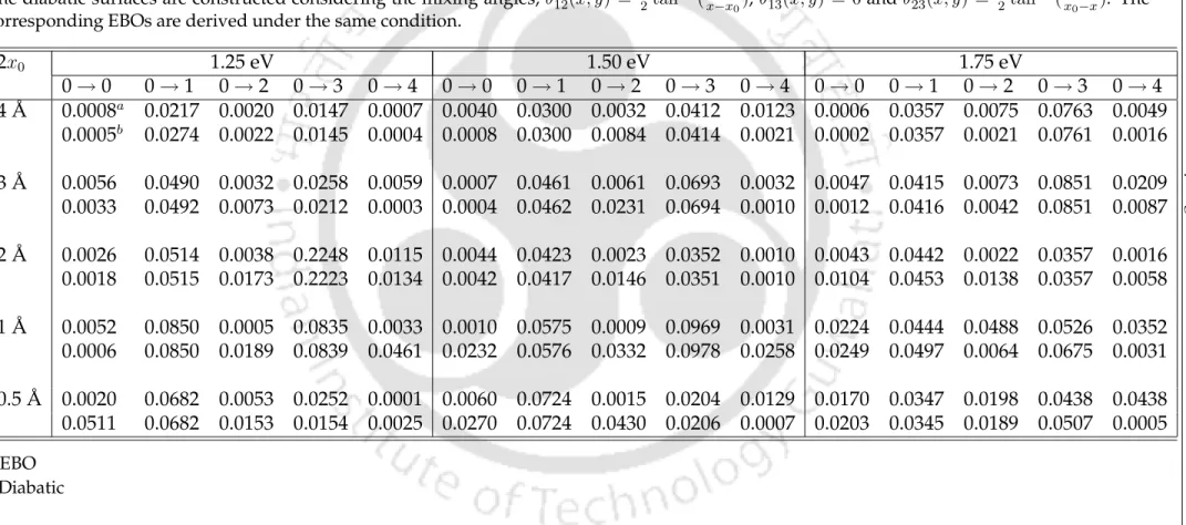
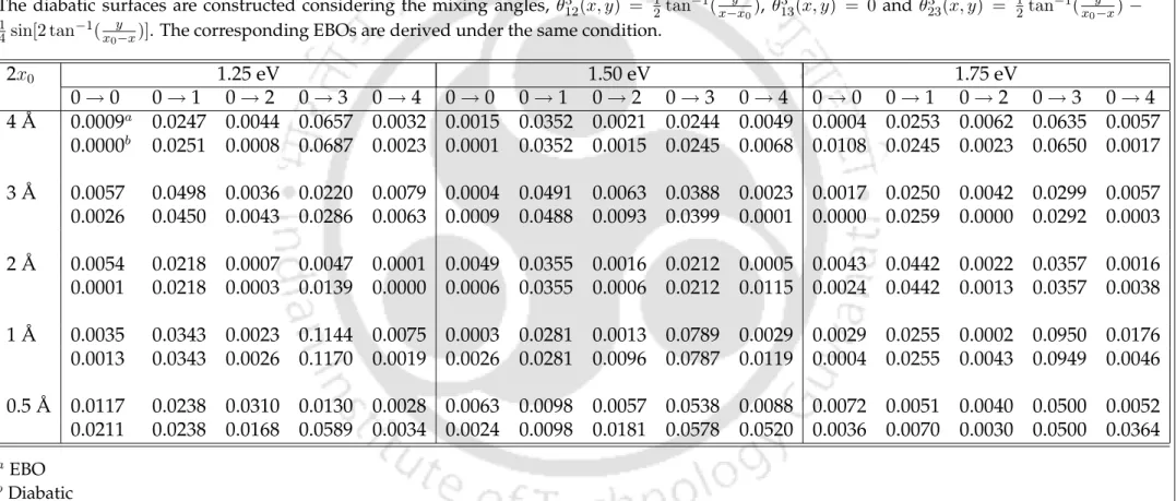
In this section, we first demonstrate1,2 the validity of our rigorous EBO equation [Eq. 2.39)] and find its necessity with respect to the estimated EBO equation [Eq. Although we obtain good agreements between the results calculated using Eq. 2.39) to include the contribution of the elements of Gmatrix. The results obtained from these equations are compared with the so-called numerically exact diabatic equation [Eq. 2.6)], where calculations are performed on two different models (Model On and Model B) involving three electronic states.
The Models and the nonadiabatic coupling elements
The Model A
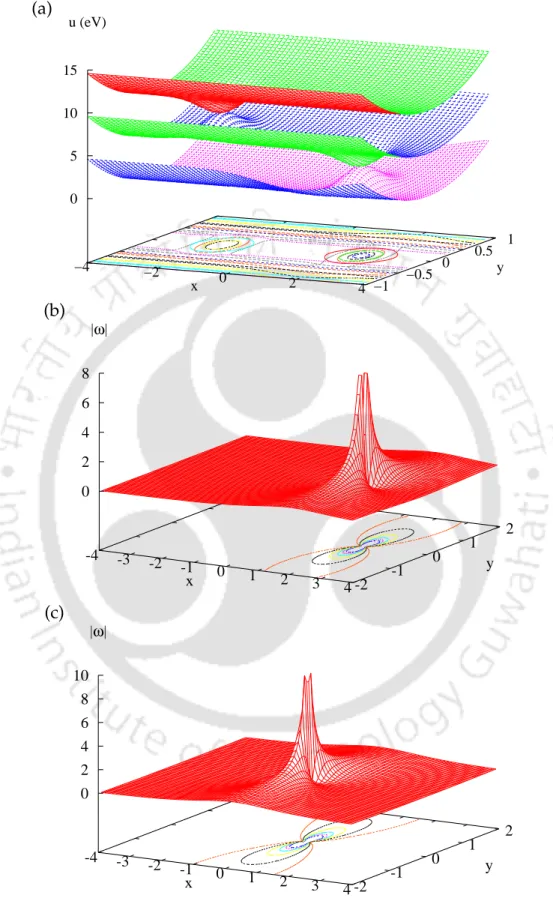
The functional form of the eigenvalue (|ω|) of the NAC matrix arising due to set (II) ADT angles is presented in Fig. This effect is more prominent with the choice of the functional form of the quantity (III) - mixing angles and Table 4.3 clearly shows this fact. On the other hand, Table 4.8 presents the reactive state-to-state transition probabilities for the set (II) ADT angles with the separation between the CIs of 4 and 0.5 ˚A, respectively.

The Model B
So we substitute the set (V) and (VII) ADT angles into the equation. 2.10) to see the spatial distributions of non-adiabatic coupling elements and present in Fig. The corresponding rigorous EBOs [Eq. 2.40), since the transformation matrix commuting with the KE operator∇~ is derived under the same condition. On the other hand, the need for a rigorous EBO comparison [Eq. 2.39] with respect to the estimated EBO equation [Eq. 2.40] can be predicted based on the following gauge invariance.
Summary
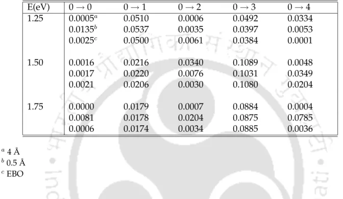
We initialize the Earth's adiabatic wave function with different initial KE as described in the case of model A, propagate the wave function, and then project the function att→ ∞ onto the asymptotic eigenfunctions of the Hamiltonian to calculate state-to-state vibrational transition probabilities. Since the point of the conical intersection between the three states is at 3.0 eV, the upper electronic states are expected to be classically closed relative to the ground at total energies and 1.75 eV, and thus the formulated approximate and stringent EBO should -equations give transition probabilities with enough accuracy. Transition probabilities when performing calculations on the single adiabatic surface with BO approximation [Eq.
The Induced Renner-Teller Type model
The nonadiabatic coupling elements and their Curl-Divergence equa-
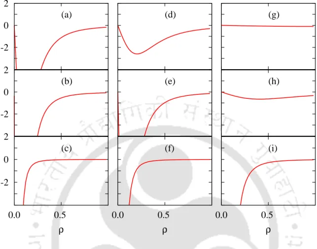
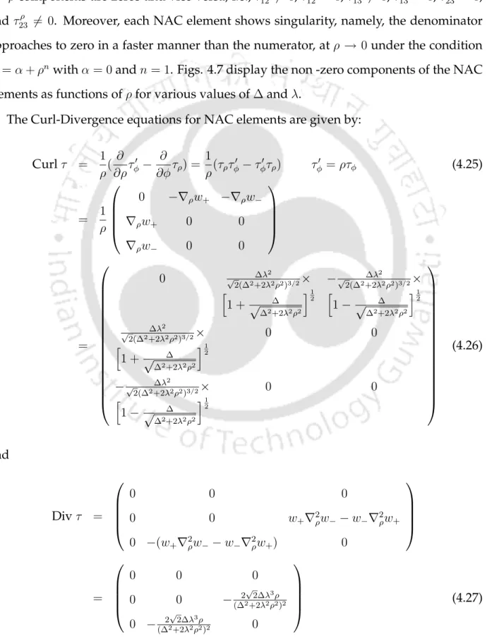
For all nonzero values of the gap,2∆, both Π states exhibit degeneracy at ρ = 0, but at ρ 6= 0 they split gradually with increasing values of λ. It is important to note that all NAC elements, both their ρ and φ components, are independent of the nuclear coordinate,φbut depend onρalong with the parameters,∆ and λ. The analytic expressions of Curls of the NAC elements show that the Curls are zeros, namely that the numerator of the Curls approaches zero faster than the denominator at ρ → 0 under the condition ∆ = α + ρn with α = 0 and n = 4.
The NAC elements at three state degeneracy and formulation of
Summary
The calculated NAC terms using the Mathieu equation provide a vast scope to explore the above two important aspects.
The Mathieu equation as the model system
This feature can affect the convergence speed for points on the real axis and therefore convergence was treated with care in each case. In this regard, it is important to mention that we have included at least 200 bases to ensure convergence, even if the required convergence comes within 50 bases.
Numerical calculations: results and discussions
Non - adiabatic coupling elements
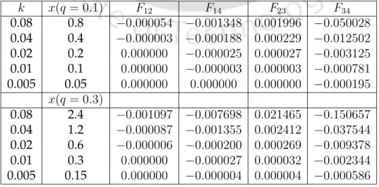
It is again quite clear from the figures that as the k value decreases for a fixed eel, both the φ and q components of the non-adiabatic coupling terms show less and less change as the functions of q lead to a progressively lower interaction among the adiabatic states. This feature of NAC terms obtained as the solution of the Mathieu equation is supported based on the calculated divergence of the same NAC terms. Figures 5.8 show the curls of the NAC elements, calculated using the equation Cij = (τφτq)ij −(τqτφ)ij. Figures 5.9 show the same quantities evaluated using the Zij equation.
Adiabatic - Diabatic Transformation (ADT) angle
At this junction we are in a position to calculate the identities (differences of the product of cross derivatives) as defined in the curl equation [Eq. Finally, since the representative four states intend to form a sub-Hilbert space for a set or sets of parameter values, the Curl and Yang-Mills fields of the NAC terms tend to zero, leading to the validity of the adiabatic equation [Eq. In this article, we only investigate the condition for finding such a sub-Hilbert space, where beyond the BO equation [Eq.
Summary
The strength of the field is measured by the number (L) of electronic states that are populated during this process.

The Schr ¨odinger Equation
The field-dressed Hamiltonian
In what follows, He(se|s, t) is assumed to contain the interaction potential formed by the field. Here He0(se|s)(= He(se|s)) is the unperturbed field-free Hamiltonian and UE(se|s, t) is the interaction formed by the field. Assuming that the electrical interaction is formed by a single electron, its potential is given by the following line integral in electronic space: 7–9.
The field-free and the field-dressed framework
Here, ω(s, t) is the matrix responsible for the transformation from the field-free manifold to the field-coated manifold. Our next step is to express the adiabatic core functions in terms of the corresponding diabatic functions [as done in the field-free case, see Eq. 6.8)], and for this purpose we use the corresponding field-coated ADT matrix A˜(s, t). The field-coated potential matrix W˜ (s, t), in Eq. 6.14), plays the same role as the field-free potential matrix W(at).
The transformation matrix, ω(s, t)
The Hilbert Subspace
The field-free Hilbert subspace
With this interpretation, it is well understood that only a limited number of countries are settled in this process. The number (-1) and their location along the diagonal reveal information about the number of CI points (i.e. degeneracy points) and their positions in a given region. Furthermore, by calculating the Dmatrix along various contours in the region of interest, we can unambiguously determine the number of CI points in that region11.
The field-dressed Hilbert subspace
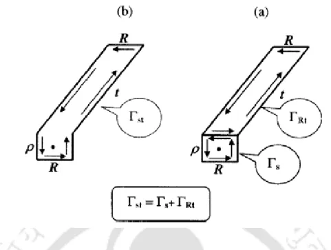
The first is a "pure" spatial closed contour (which forms a spatial region), and the second is a space-time contour (which forms a space-time region). b) The closed space-time contour Γst (follow the arrow) consisting of two space coordinatesR andρ and one time coordinate. Corollary: A space-time region formed by an open spatial contour does not contain singularities. If a closed space-time region contains singularities, they must be located only in the closed spatial region.
The square case: N = L
We remember that since all the matrices (namely τ,ω,H˜e,τ˜,H˜˜e andA˜) mentioned in Eq. 6.17) is of dimension N ×N, the unknown matrix A˜ can be presented as a product of two N-dimensional matrices. whereω is introduced in Eq. 6.17a) and recalling the definition ofτ˜[see equation(6.12)], we obtain after a few algebraic operations that this is a solution of the first-order (field-free) vector equation. To check that we substitute Eq. 6.15), we find that this substitution leads to the first-order equation for ω, as given in Eq. Equation (6.42) implies that in the case of L = N the space-time ADT matrix A˜(s, t) is written as a product of the matrix ω†(s, t) and the field-free ADT matrixA(s) ).
The Mathieu Equation
In the case of a perturbative framework, the diabatization yields the identical potential matrix W(s, t) as given in Eq. When the general (non-perturbative) approach is performed for N = L, the resulting diabatic potential matrix is identical to that obtained in the simplified perturbative approach. It is important to emphasize that all degeneracy points (i.e., CI points) produced by Mathieu's equations are located at q = 0.
The External Electric Field
The (electronic) potential
Since E is an external field formed outside the molecular region, E must satisfy two equations in electronic coordinates (as well as in atomic coordinates): curlE=0 and divE=0. This choice can be used to show that the angular component of the field. In the following, we assume short pulses so that σt, the quantity responsible for the width of the normal distribution, is narrow enough (it does not matter for the value of t0) to ensure that at both ends of the time interval, namely t = 0, T, we have E (t)˜ ~0.
The nuclear dressed-field potential
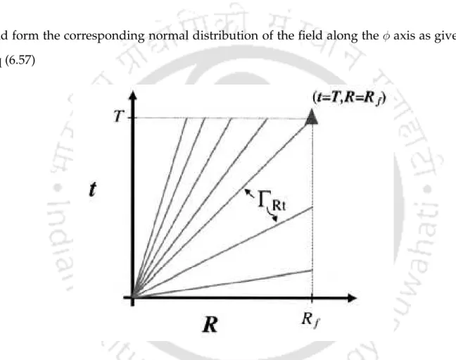
Therefore, the first difficulty to be solved is to reveal a characteristic space-time contour along which D˜ matrices are to be computed. The advantage of using Eq. 6.58) is not only because it transforms a normal distribution in time into a normal distribution in space, but also because it defines a line that can become a segment, ΓRt, for a (closed) space-time contour. Then, to close the space-time contour, we need to add a second segment, Γnamely, {(t=T, φ = 2π)→(t= 0, φ= 2π)}which is a segment along the negative time axis.
Numerical Results
- Introductory comments
- Numerical treatment of the ω matrix and the corresponding elec-
- Numerical treatment of the field-dressed NACMs
- Numerical treatment of A ˜ : The ADT field-dressed matrix
Details about solving the first-order differential equation for the ω matrix are given in Appendix E. Since the elements of the ω- matrix are complex numbers, we focus only on their norms. The situation worsens for the perturbative approach in the second example because now the two missing elements of the matrix P account for almost 50% of the transition probability see Fig.
Summary
In other words, regardless of how intense the field is or how long it operates, it cannot affect the topological features of the field-free Dmatrix. Here, the difficulty to worry about is related to the singular value of the calculated diabatic potentials. The first terms in Eq. B.6) is zero due to the analyticity of the ADT angle (θ12), and the second term is automatically zero.

![Figure 4.4: Profile of the nonadiabatic coupling elements, (a) τ 12 , (b) τ 23 and (c) τ 13 for the adi- adi-abatic - to - diadi-abatic transformation angles angles θ 12 (x, y) = − 2 sin 2 [ 1 2 tan −1 ( y x )] , θ 13 (x, y) =](https://thumb-ap.123doks.com/thumbv2/azpdfnet/10465081.0/98.892.177.736.153.994/figure-profile-nonadiabatic-coupling-elements-abatic-abatic-transformation.webp)