The effect of intrinsic decay can be significantly reduced by using the TQD protocol. The robustness and almost perfect accuracy of adiabatic processes are preserved in these STA techniques.
The adiabatic theorem
Therefore, here we invoke the adiabatic approach by choosing the external field to vary slowly, which can be mathematically expressed as The adiabatic state: To properly understand the adiabatic approximation, let's go back to Eq.
Adiabatic passage: A demonstration of adiabatic theorem
At the beginning of the frequency sweep, Δ(t) < 0 and the adiabatic state |Φ+(t)� corresponds to the diabatic state |1�. So it is clear that the frequency change rate should be very small compared to the strength of the external field.
Shortcut to adiabaticity
Transitionless quantum driving
According to this method, the transition probability between current eigenstates can be set to zero to make the time evolution accurate. The newly designed Hamiltonian H�(t) drives the adiabatic states along the adiabatic path, but without creating any transition probability between them.
Lewis-Riesenfeld invariant based approach
In general, for a particular invariant, there may be many possible Hamiltonians based on the choices of αn(t). In fact, as a consequence of the existence of αn(t), the eigenstates of H(t) and I(t) do not coincide. So, to drive the system from an initial HamiltonianH(0) to a final H(tf) such that the populations at the initial and final instantaneous basis are the same, we must impose [H(0), I H( tf ), I(tf)], so that both H(t) and I(t) share the same eigenstates at least at the boundaries.
In physical applications, the Hamiltonians H(0) and H(tf) are given and we set the initial and final configuration of the external parameters. As for the exact evolution of the adiabatic states, it does not matter, since at the end of evolution one gets the desired final state.
Chapter summary
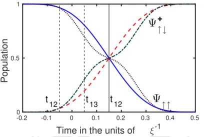
In the recent past, few works have shown that adiabatic tracking can be successfully performed to prepare complex states. They considered the combination of a pair of two-state systems consisting of two particles with spin 12 connected by an internal exchange interaction and an external time-dependent magnetic field. If we choose these four states as a basis, we can easily study the adiabatic evolution of this system.
However, the issue of long preparation time, inherent in the adiabatic passage method, still exists. Here we study the possibilities for the preparation of entangled states in a coupled spin pair system using the shortcut techniques.
Adiabatic method
These can be easily recognized as triplet and singlet states in which |ψ↓↑+�in. Therefore, when studying the dynamics of the system, |ψ−↓↑� can be neglected, and the effective Hamiltonian can be written as,. Since the magnetic field is time-dependent and contributes to the diagonal and off-diagonal terms of the interaction Hamiltonian, its choice is crucial.
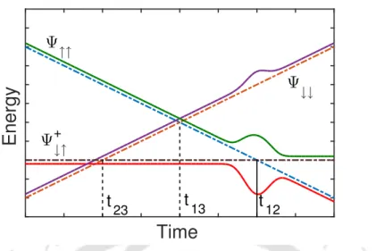
Adiabatic energies are shown with solid lines and diabatic energies with dashed lines. 2 In fact, the dashed lines and the corresponding solid lines coincide with each other except at t12.
Transitionless quantum driving
Therefore, we can further simplify our system by eliminating the contribution of |ψ↓↓� from HI(t). 3.2a), we numerically plotted the population of the entangled state |ψ↓↑+� while varying α and Ω0. However, when the adiabatic condition is not met, no exchange of populations takes place at all for Q=2. According to Berry's algorithm of transitionless quantum propulsion, it is always possible to construct a driving Hamiltonian, which cancels out the non-adiabatic part of the adiabatic Hamiltonian.
The interaction time has been scaled down to 1% compared to that required in the adiabatic case. This causes violation of the adiabatic condition as the Q value goes up to as high as 50.

Lewis-Riesenfeld Invariant based approach
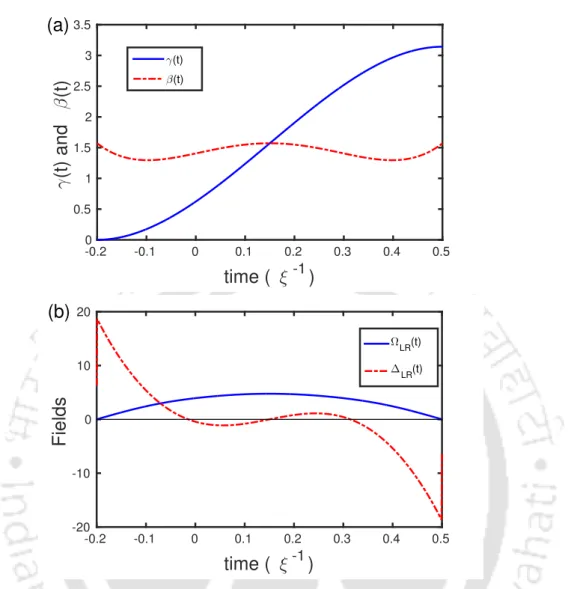
To invert this system we design I(t) by the parameters γ(t) and β(t) with specific boundary conditions so that it commutes with HI(t) at least at the beginning and at the end of the evolution, i.e. . These choices are completely consistent with our choice of the external field for adiabatic evolution. The dynamics of the Hamiltonian follows an adiabatic path while the invariant does not, but the end results are the same for both cases.
However, in the case of other two methods fidelity is close to unity regardless of the total transition time which is again well beyond the adiabatic condition. The TQD approach shows a value up to F = 0.999, while in the case of the LRI-based approach fidelity is even closer to unity.
Chapter summary
- Coupled mode theory
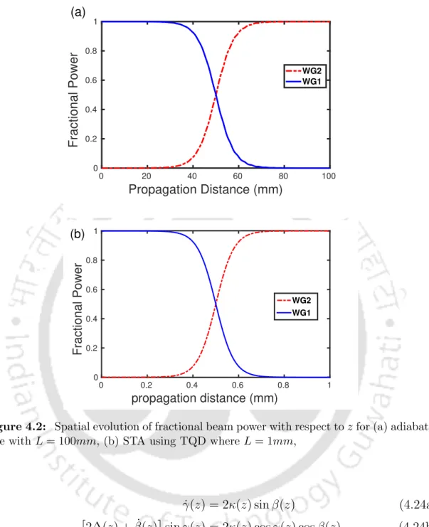
- Adiabaticity in two waveguide coupler
- TQD in two waveguide coupler
- Invariant based STA in two waveguide coupler
- Results and discussion
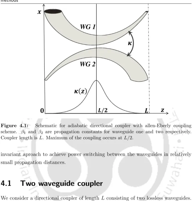
Now let Ψ(x, y, z) be the total field of the entire structure of the directional coupler with a weak interaction between the waveguides. The coupler geometry depends on the mutual coupling between the waveguides and the mismatch coefficient. On the other hand, the narrowing of the waveguides is controlled by the mismatch coefficient.
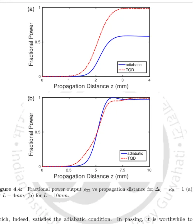
However, the discrepancy is much larger in the case of the invariant method compared to the TQD technique. It accurately shows the adiabatic nature of the evolution, but requires very small coupler lengths to complete the power transfer.
Three waveguide coupler
4.6) shows that the strength of the couplings determined with the L-R invariant method is almost the same as what we determined with the TQD (Fig. Regarding the practical implementation of the scheme, one can use a Silica ( SiO2) based fiber coupler[136] that uses the proposed scheme can be engineered with judicious choice of the core radius, the center-to-center separation between the waveguides, and the refractive index difference between the two waveguides.
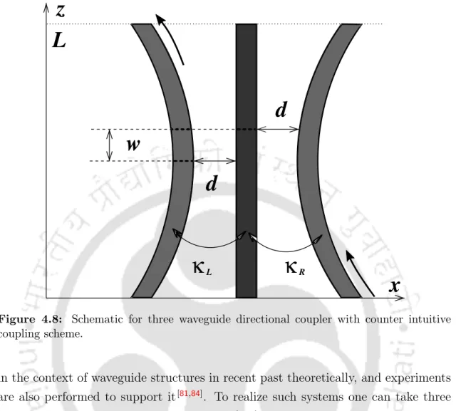
The minimum distance d between the curved and the straight waveguide is displaced by a distance w to make the counterintuitive coupling plausible, as shown in Fig. The power development in Fig. 4.10a) shows that, for such configuration, power switching can be achieved with very short propagation distances, ultimately leading to the minimization of coupler length. 4.10b) shows the coupling efficiency with varying device lengths and the output power remains close to unity regardless of the length of the coupler, while the efficiency for the adiabatic approaches unity only for large lengths.
Chapter summary
In this work, we also take solitary wave and soliton to have the same meaning. In this regard, a particular study worth mentioning is that of Jing Liet al., where they proposed a method to achieve controlled compression of soliton matter waves in harmonic traps by tunable interaction using STA[110]. In this work, we propose for the first time to the best of our knowledge a scheme to achieve temporal soliton compression in a nonlinear waveguide of arbitrarily small length by using the shortcut adiabatic passage technique.
The scheme proposed in this work is a combination of the Lagrangian variational approach with STA, which was first proposed by Jing Li et al. [110] was introduced. in the context of soliton matter waves. In this work, authors proposed a scheme to compress soliton by designing the dispersion but keeping the nonlinear coefficient constant.
The model and theory
Variational analysis
In this section, we use the variational method to study the dynamics of the soliton width[151-153]. It should be noted that δLδφ = 0 , which means that φ plays no role in the variational dynamics, and therefore we set φ= 0 in the rest of the work. It is obvious from the above equation that the width of the solitary wave, α, is dependent on the Kerr parameter γ.
Compression via adiabatic process
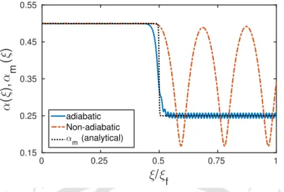
The minimum achievable soliton width, αm(ξ), depends explicitly on the nonlinearity function γ(ξ) and gives us an estimate of the compression that can be achieved with adiabatic compression. It is found that α(ξ), the solution of Eq. 5.7) adiabatically coincides with the minimum value αm(ξ). 5.1) shows the evolution of the soliton time width as a function of distance for the adiabatic and non-adiabatic cases.
Here we compare the exact result obtained by Eq. 5.7) with the adiabatic reference given by Eq. We see that the exact result is close to the adiabatic result; the pulse is compressed from its initial value α = 0.5 to α = 0.25 after propagating a distance, ξ = 50, for the chosen parameters.
Compression via inverse engineering
However, this may not be realistic as illustrated in Fig. 5.3), which depicts the non-linear profiles for different lengths of the fiber. It is easy to observe that as one reduces the length of the fiber, the corresponding inverse nonlinear profile may no longer remain smooth enough for practical implementation. It can also be noted that to compress a soliton over a very small distance, one must increase the optical power of the input pulse.
This is because, the dispersion length is inversely proportional to the input peak power of the fundamental soliton; for a fundamental soliton N=1. Finally, to get an idea about the usefulness of the proposed scheme, let us consider a silica optical fiber with β2 = -20ps2/km[145].

Chapter summary
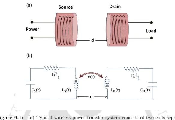
However, the recent tide in the use of electronic devices and the need for short- and medium-range wireless energy exchange have caused WPT to receive immense attention, and studies on WPT systems have gained momentum in recent years [160,161 ]. In a recent seminal paper [113], Soljaˇci´c's group experimentally demonstrated non-radiative force transfer over a reasonable distance, using self-resonant coils in the strong coupling regime. WPT also depends on the coupling distance between the coils and it has been shown in a few papers that in the strong coupling regime it is possible to improve the efficiency for greater distances.
Using the coupled mode theory [170], we find the governing equations (which are similar to the Schrödinger equation for two-level systems) and design a power transfer mechanism that is insensitive to the coupling strength and spacing between the coils and intrinsic losses present in the system. In the rest of the analysis we only look at the positive frequency component and omit the '+' subscript for simplicity.
Energy transfer protocols
Adiabatic following
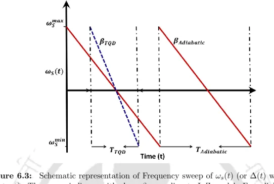
For adiabatic evolution, one must change the Hamiltonian infinitely slowly or adiabatically so that the system always follows a particular state B+ or B- during a complete cycle of the time evolution. Under such choices, large t0 is required to satisfy the adiabatic condition and this effectively determines the width of the evolutionary cycle. However, in adiabaticity-based techniques one should usually have good control over the temporal dependence of the Hamiltonian.
When the loss rates are non-zero in both the source and the drain coil, the system can be considered dissipative. The fast and efficient transfer of wave energy via transitionless quantum conduction must be smaller than the coupling strength κ0, otherwise evolution would not be possible and power would be lost from the spiral itself.
Shortcut to adiabaticity
Results and discussion
However, it may be appropriate and relevant to briefly discuss the energy costs associated with the implementation of the proposed scheme. The coupling energy required for adiabatic power transfer will be of the order of the difference of the resonance frequencies of the source and drain coils, i.e. Δ=ωd−ωs. It is important to note that the quantification of time-energy costs in Eq.
We calculated the ratio of the energy costs for adiabatic and additional interaction, ΣT QD/ΣAd for the coupling strength parameter used in this work. On the other hand, inductance depends mainly on the orientation and the geometry of the coils.
Chapter summary
In this thesis, STA methods are used for the first time for soliton compression in optical fiber and wireless power transfer. Muga, Optimally robust shortcuts to population inversion in two-level quantum systems, New Journal of Physics. Chen, Shortcuts to adiabatic passage for the generation of W states of distant atoms, Quantum Information Processing.
Song, Entangled state generation via adiabatic passage in two distant cavities, Journal of Physics B: Atomic, Molecular and Optical Physics. He et al., Efficient shortcuts to adiabatic transit for generation of three-dimensional entanglement via transitionless quantum propulsion, Sci.