I am thankful to all the faculty members of the Department of Mathematics, IIT Guwahati for their help and support. I am thankful to all the technical and non-technical staff in the department for their help and cooperation throughout my research period.
Abstract
Introduction
Notations
Rn and Cn denote the vector spaces of real and complex column vectors of length n, respectively. I and 0 denote the identity matrix and null matrix, respectively, of appropriate size determined by the context.
Preliminaries
Then P(z) belongs to the complex vector space of all n×n matrix polynomials of degree at most m according to ordinary addition and scalar multiplication. The following definitions from the theory of non-negative matrices play an important role in the calculations of inclusions of eigenvalues in the thesis.
Literature survey
- Localizing eigenvalues of matrices and matrix polyno- mials
- Outer approximations of pseudospectra of block trian- gular matrices
34] If a diagonally dominant type class of matrices K is a class of nonsingular matrices, then it is a subclass of the nonsingular H matrices. The eigenvalue inclusion set corresponding to the class of nonsingular H-matrices is the minimal Geršgorin set.
Inner approximations for pseudospectra of block triangular matrices
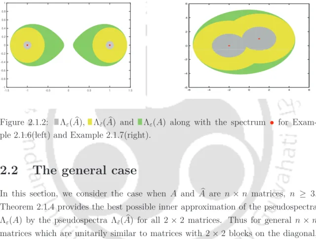
The 2 × 2 case
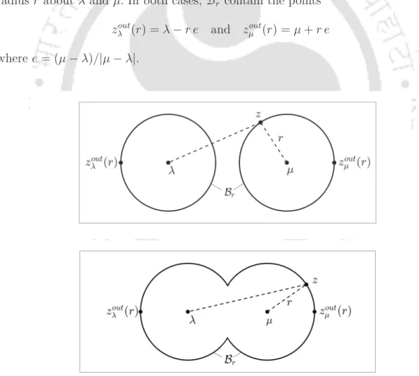
If σmin(λ, µ, c) and σmax(λ, µ, c) are respectively the maximum and minimum singular values associated with the matrix A in (2.1.1), then. 2.1.4) Both numbers are equal to the non-negative zeros of the polynomials. To prove Theorem 2.1.4, we first determine the maximum value of the function σmin(A−zI)forz ∈Br, the limit of D(λ, r)∪D(µ, r).
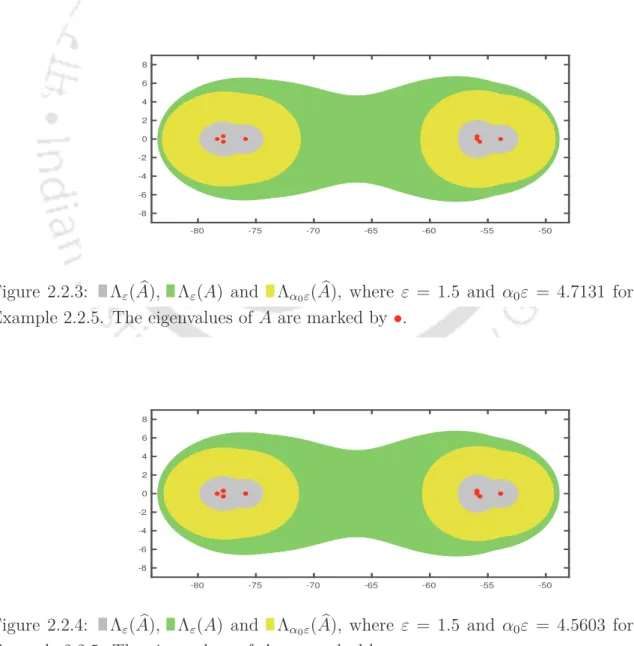
The general case
We are looking for the corresponding centrrez0 and radiiRL(α1), RM(α) for disks containing αε-pseudospectra of diagonal blocks. One strategy is to choose zˆ0 as the center of the smallest disk containing the eigenvalues of the matrix M. We choose z0 and zˆ0 to be the center of the smallest disk containing the eigenvalues L and M, respectively.
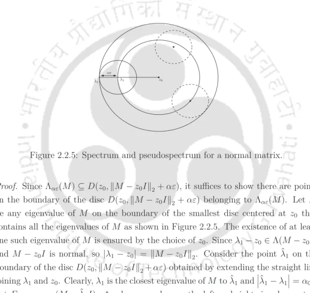
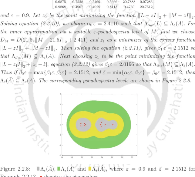
The general case If M is a normal matrix and zˆ0 is chosen as the center of the smallest disk containing the eigenvalues of M, then D(ˆz0,ëM −zˆ0Ië2 +αε) is also the smallest disk containing Λαε(M) . Let M ∈ Cm,m be a normal matrix and let z0 ∈ C be the center of the smallest disk with the eigenvalues of M. Then D(z0,ëM −z0Ië2+ αε) is the smallest disk with Λαε(M). To use the idea of the proof of Theorem 2.2.8, to find ε > ε˜ such that Λε˜(M)⊆Λε(A)when L,M and C are as assumed in the statement, it is necessary to make sure that Cvmin(z)Ó= 0 for each straight singular vector vmin(z) of M−zI corresponding to σmin(M−zI)forz /∈Λ(M).
In cases where none of the z ∈ Λε(A) satisfies this condition, it may be possible to have an inner approximation of Λε(A) via Λαε(M) for some α >1.
Localization sets for eigenvalues of homogeneous matrix polynomials
Block Geršgorin-type localizations for eigen- values of homogeneous matrix polynomials
- Approximating the block Geršgorin and block minimal Geršgorin sets via pseudospectra
- Equivalent characterization of block minimal Gerš- gorin sets for matrix polynomials
The block Geršgorin set for the homogeneous matrix polynomial P(c, s) (as in (3.1.1)) with respect to the partition π ={nj}üj=0, is defined as. We now establish the following properties for the block Geršgorin set of the matrix polynomial P(c, s). The block minimal Geršgorin set for P(c, s) with respect to partition π and norm ë·ëp, denoted by HGπp(P) is defined as.
As in Theorem 3.1.2, it is easy to verify the following properties for the block-minimal Geršgorin set. In fact, they can be seen as an alternative definition of Geršgorin's minimal sets, since the two sets can be determined to be equal. Then the block minimal Brualdi set for the homogeneous matrix polynomial P(c, s), denoted Hβpπ(P), is defined as.
The block of Brauer groups for the matrix polynomial P(c, s) partitioned as in (3.1.2) with respect to each p-norm of the induced matrix is defined as follows.
Permuted pointwise minimal Geršgorin set for homogeneous matrix polynomials
If the premultiplication of T interchanges rows i and j of the comparison matrix éP(c, s)êπp, then the same block and j rows of the blocked matrix [Pk,j(c, s)]ü×ü are interchanged. inT Pâ (c, s). Similarly, if post-multiplication with T changes the columns of andj to TéP(c, s)êπp, then the same block of columns andj will be changed via post-multiplication of T Pâ (c, s) with Tât. Equivalent characterization of the group HΓφ(P) Here we adapt the procedure in [43, 76] for deriving an equivalent criterion that a (c, s) ∈ S is inside the group HΓφ(P).
By the Perron-Frobenius Theorem [Theorem 1.2.2], it has a non-negative eigenvalue ρ(Rφ(c, s)) and a corresponding eigenvectorxˆ∈Rn with xˆ≥0. 3.2.4) where μφ(c, s) being a continuous function of the inputs of Qφ(c, s) is in turn a continuous function of (c, s). Let Aisicm be an×n polynomial of the homogeneous matrix and let Φ be the set of all permutations in the set {1,2,. HΓφ(P) if and only if the rightmost eigenvalue of -éAmTφê is nonnegative for every nontrivial permutation φ ∈Φ.
HΓφ(P) if and only if the rightmost eigenvalue of −éA0Tφê is non-negative for any non-trivial permutation φ ∈Φ.
Plotting eigenvalue localization sets for matrix polynomials
- Numerical Experiments
Plotting eigenvalue localization sets for matrix polynomials pointwise minimal Geršgorin set is equivalent to the minimal Geršgorin set. The projections of the block minimal sets of Geršgorin (or the block Brualdi sets) on the complex plane are shown in Figure 3.3.7. The pointwise Geršgorin set [52] and the pointwise minimal Geršgorin set are shown in Figure 3.3.6 (right) and Figure 3.3.8 (right), respectively.
The block Geršgorin set plotted on the Riemann sphere is shown in Figure 3.3.9 (left), and its corresponding projection on the complex plane can be seen in Figure 3.3.9 (right). Therefore, we plot the permuted pointwise minimal Geršgorin set, which can be seen in Figure 3.3.11. We plot the projection of the pointwise Geršgorin set and the pointwise minimal Geršgorin set onto the complex plane in Figure 3.3.16 (left) and Figure 3.3.16 (right), respectively.
The permuted pointwise minimal Geršgorin set is identical to the block-minimal Geršgorin set.
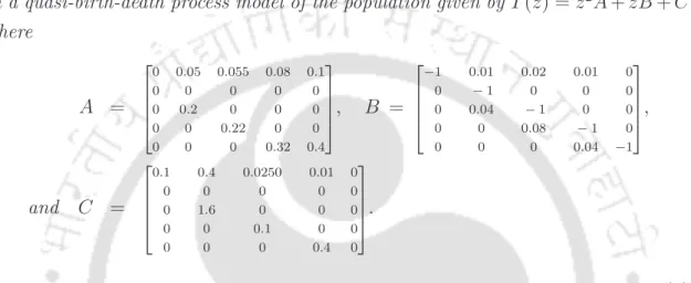
Applications of block Geršgorin sets arising from linearizations of quadratic matrix polynomials
Linearizations of matrix polynomials arising from vector spaces
Block Geršgorin sets arising from lineariza- tions of quadratic matrix polynomials
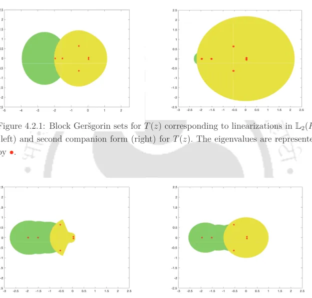
With this partitionπen induced operator norme.ëp, for the sake of simplicity, we denote throughout this chapter the block Geršgorin set Γπp(L) obtained via the linearization L(z) of P(z) by the notation Γ(P ). To determine whether the eigenvalue ∞ belongs to the set R1 or R2, we look at the block Geršgorin set resulting from revL(z) given by. It is clear from Theorem 4.2.1 that if the pencil zA2+A1 is singular, then the block of Geršgorin sets corresponding to the first and second companion forms is the entire complex plane.
The block Geršgorin series in theorems 4.2.1 and 4.2.3 are obtained by linearization with respect to the anzatz vectors αe1 and αe2, where α∈C\{0}. We now consider the general case of an anzatz vector v that is not a multiple of e1 ore2. Therefore, when R1 and R2, as in Theorem 4.2.4 and Theorem 4.2.5, are constructed with such choices of W1 and W2, their block of Geršgorin union forms sets Γ(P), which can be connected to infinitely many linearizations in L1(P ) or L2(P). Since DL(P) = L1(P)∩L2(P), it is natural to expect that the block Geršgorin set R1∪R2 given in Theorem 4.2.7 is a special case of the sets R1 and R2 obtained earlier with respect to strong linearizations in L1(P) and L2(P).
In view of Remark 4.2.8, Geršgorin block groups arising from linearizations in DL(P) are special cases of those arising from linearizations in L1(P). So it suffices to prove the theorem for strong linearization L(z) ∈L1( P).
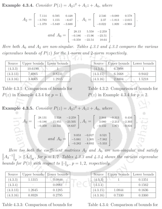
Bounds for eigenvalues of quadratic matrix polynomials
Bounds for the eigenvalues of the quadratic matrix polynomials can be obtained by choosing W2 = 0 and W1 to be any non-singular matrix in (4.3.2) and (4.3.1) respectively applied to revP(z). If the linearization in L1(P) corresponds to the ansatz vector αe1, then the corresponding Geršgorin block group R1 ∪R2 is given by theorem 4.2.1(iii) and due to theorem 4.2.10, all upper and lower bounds on the values eigenvalues of P(z) arise by considering the set R1 for P(z) and revP(z). Arguing both in the proof of Theorem 4.3.2 and in the previous lines of this remark, the optimal upper and lower bounds on the eigenvalues of P(z) obtained by this approach are those for which W1 = 0 and in fact are u1 and l1.
Therefore, if we apply Theorem 4.2.10 and inequalities in Lemma 4.2.9, then l1 and u1 are the optimal eigenvalue bounds of P(z) arising from block Geršgorin quantities associated with strong linearizations of P(z) in L1 ( P) with respect to the natural partition induced by the linearization. Limits for eigenvalues of square matrix polynomials The limits in Theorem 4.3.2 are easy to calculate. Most of the upper bounds are obtained by assuming that A2 is non-singular and considering the matrix polynomial PU(z) :=Iz2+U1z+U0 where. 4.3.11) The following bounds were obtained in Lemmas 2.2 and 2.3 of [28] by considering the first accompanying linearizations, CU(z) and CL(z) of PU(z) and PL(z), respectively.
Bounds for eigenvalues of quadratic matrix polynomials show that if min{u1, u2} and l1 in Theorem 4.3.2 are close to their optimal value (which is 1), then they can be quite close toup and lp from (4.3.16). .
What do coefficient matrices of quadratic ma- trix polynomials reveal about their eigenval-
Since R1 and R2 come from the first accompanying linearization, according to Theorem 4.0.1, the number of eigenvalues of P(z)inD is equal to the number of eigenvalues of the matrix pencil zIn andD when counting multiplicities. If any of the following conditions hold, then P(z) has no eigenvalues on the unit circle. Thus, if any of statements (i), (ii) and (iii) hold, then by Theorem 4.4.1(ii) P(z) has n eigenvalues in Dc. Due to the grouping of eigenvalues, the remaining eigenvalues P(z) fall inside D.
The number of eigenvalues of Q(µ) in Dc, the interior of D and on the unit circle excluding -1 are equal to the number of eigenvalues of P(z) in the open right half of the complex plane, the left half open to the complex plane and to the imaginary axis, respectively. Then P(z) has no purely imaginary eigenvalues if any of the following holds. The proof follows from Corollary 4.4.5, due to the fact that every λ ∈ R is an eigenvalue of P(z) if and only if iλ is an eigenvalue of the even polynomial ∗ .
Therefore, the conclusions can be restated in terms of P(1), P(-1), P(i) and P(-i). In fact, the quantities in the LHS of the inequalities in Corollary 4.4.4 (i) and Corollary 4.4.4(ii) are proportional to the lagged errors of 1 and −1 respectively taken as approximate eigenvalues of P(z), the constant of proportionality is a function of the choice of norm in P(z) (see for example, [1]).
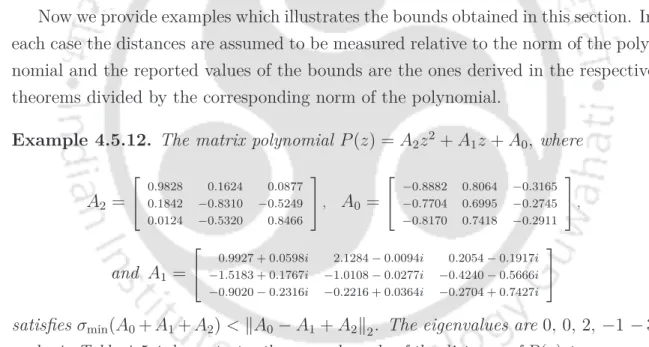
Upper bounds on some distances associated with quadratic matrix polynomials
Therefore, according to 4.4.4(i), (P +δP)(z) has no eigenvalues in the closed right half of the complex plane. 2) which completes the proof of this case. Since P(z) has an eigenvalue in the closed right half of the complex plane, by Corollary 4.4.4(i),F(P)≤0. The proof in this case is complete by showing the existence of a polynomial δP(z) of degree two such that (P +δP)(z) ∈ Pn has no eigenvalues in the closed right half of the complex plane and | || δP|||∞,1 < ε.
Then the distance to a nearest matrix polynomial of the same structure that does not have any purely imaginary eigenvalues with respect to the norm |||·|||2,2 is bounded above by ëA0+A1+A2ë2−|λmin(A0−A2 ) |. However, if the distances are measured in a relative sense with respect to the norm of the polynomial, then the differences in the upper bound values with respect to such differences are reduced. In this thesis we have studied various aspects of localization groups for spectra and pseudospectra of matrices and matrix polynomials.
Finally, we studied the localization sets for the eigenvalues of polynomials of square matrices using the concept of block Gershgorin sets applied to polynomial linearizations.
Bibliography