Types, Number And Dimension Synthesis
Graphical And Analytical Synthesis
The number of precision points that can be synthesized is limited by the number of equations available for solution. The four-band connection can be synthesized by the closed-form method up to 5 points precise for the generation of the timed path. The graphical procedure used for the two-position synthesis problem can be extended to three-position synthesis.
Six of them are defined in the problem statement, 2 can be chosen freely.
Coupler Curves
This equation describes the coupling curve for a four-link mechanism, which is of sixth order. The shape and state of the coupling curve changes with the changing positions of the coupling point P. The coupling curve is said to have double points when the coupling point P passes through the same position twice as shown in fig.
So, as the coupling rotates around the top, the coupling point changes its direction of motion.
Cognates And Roboerts-Chebychev Theorem
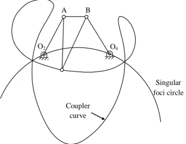
The applications of the coupling curves for a four-bar connection are found in the film advance mechanism of the movie camera projector, car suspension systems, etc. Now construct the lines parallel to all sides of the links in the original connection to create a Cayley diagram (Fig.1.7) ). All three four-bar links share the original coupling point P and generate the same path motion on their coupling curves.
To find the location of the pivot O3 from the Cayley diagram, the ends of links 2,4 are returned to the original locations of the fixed pivots O1 and O2.
Literature Review
Objectives Of Present Work
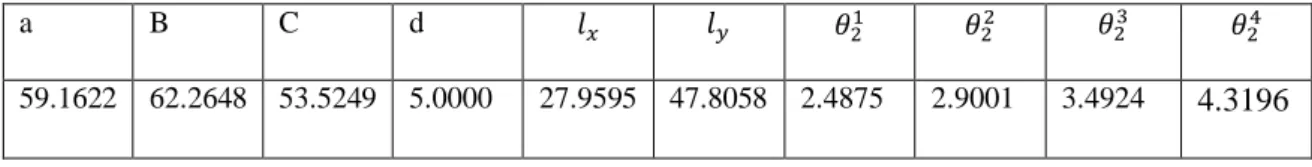
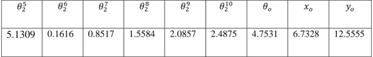
To trace the coupling point, the dimension of the links (a, b, c, d, Lx, Ly) must be determined together with the input crank angle θ2, so that the average error between these specified precision points (Pxdi, Pydi) ), ( where i=1,2,…N with N given as number of precision points) and the actual points to be traced by the coupling point P are minimized. The synthesis of the four-measure mechanism largely depends on the choice of the objective function and the equality or inequality constraints imposed on the solution to obtain the optimal dimensions. In general, the objective function is minimized under certain conditions so that the solution is satisfied by a set of the given constraints.
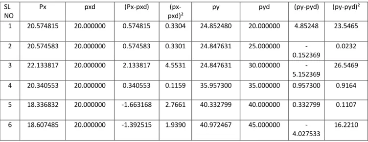
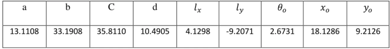
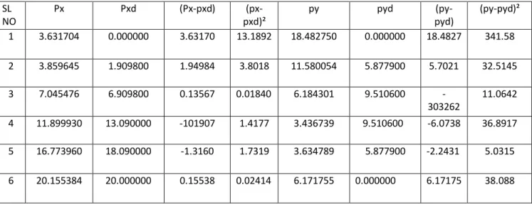
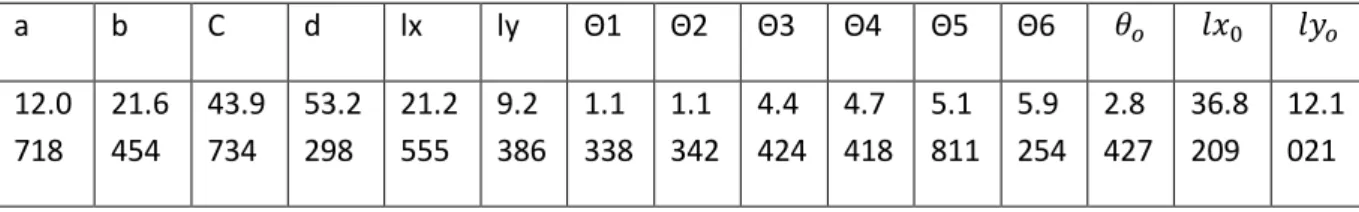
Grashof criterion states that the sum (Ls+Ll) of the shortest and the longest links must be smaller than the sum (La+Lb) of the remaining two links. For constrained problems, most applications use penalty function method which transforms objective function f(X) into an unconstrained function F(x) consisting of a sum of the objective and the constraints weighted by penalties. The synthesized geometric parameters and the corresponding values of the precision points (Pxd, Pyd) and the tracked points through the coupling point (Px,Py) and the difference between them are shown in table 1 and table 2, respectively.
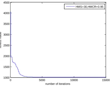
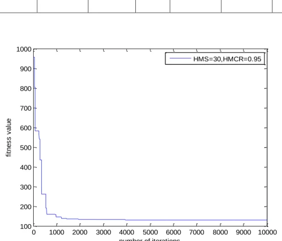
The synthesized geometrical parameters and the corresponding values of the precision points (Pxd, Pyd) and the points tracked by the connection point (Px,Py) and the difference between them are shown in Table 3 and Table 4, respectively. Although the limitation of the sequence of input angles during evolution is ignored in this case. The accuracy of the solution in case 1 is significantly improved using the present method. fig (4.4) shows the ten target points and the coupler curve obtained using the harmonic memory search method with NVAR=18, Maxitr=10000, HMS=30, HMCR=0.95, PARmax=0.9, PARmin. The synthesized geometric parameters and the corresponding values of the precision points (Pxd, Pyd) and the points tracked by the tie point (Px, Py) and the difference between them are shown in Table 5 and Table 6, respectively.
Although the constraint of the order of the input angles during the evolution is ignored in this case. The synthesized geometric parameters and the corresponding values of the precision points (Pxd, Pyd) and the tracked points through the coupling point (Px, Py) and the difference between them are shown in table 7 and table 8, respectively.
PATH SYNTHESIS OF FOUR-BAR LINKAGE
Position Error As Objective Function
Some authors have also considered additional objective functions such as the deviation of the minimum and maximum transmission angles min and max from 90o, for the entire set of initial solutions considered.
The Constraints Of The Linkage
An objective function is usually used to determine the optimal link lengths and joint geometry. For path synthesis problems, this part is a sum of squares that calculates the position error of the distance between each calculated precision point (Pxᵢ, Pyᵢ) and the desired points (Pxdᵢ,Pydᵢ), which are the target points specified by the designer. where X is the set of variables to be obtained by minimizing this function. There are usually large combinations of mechanisms that generate coupling curves that pass through the desired points, but these solutions may not satisfy the desired order.
To ensure that the final solution respects the desired order, testing is implemented for any order violations. This is achieved by requiring that the direction of rotation of the crank is determined by the sign of its angular increments. For a locking mechanism, generally the best results, designers recognize when the transmission angle is as close to 90 degrees as possible throughout the rotation of the lock.
Alternatively, the transmission angle must lie between the minimum and maximum values during the entire rotation of the crank. That is, the non-dimensional constraint variance is added directly to the objective function for minimization. All variables considered in the design vector must be defined within pre-specified minimum and maximum values.
For example, if we have 19 variables in a 10 point optimization problem, all the variables can have different values of minimum and maximum values. Generally, in non-conventional optimization techniques starting with set of initial vectors, this constraint is handled at the beginning itself, while defining the random variable values.
Overall Optimization Problem
Minimize f(X) subject to xiX, i=1, 2..N (3.1) Where f(X) is an objective function; X is the set of decision variables; N is the number of the decision variable; X is the set of possible ranges of values for each decision variable, i.e. xi. HMCR, which varies between 0 and 1, is the rate of selecting one value from the historical values stored in HM, and (1-HMCR) is the rate of randomly selecting one value from the possible range of values. 3.2) The value of each decision variable obtained by taking memory into account is examined to determine if it needs to be adjusted in height. If the new harmony vector is better than the worst harmony vector in the HM, based on the evaluation of the objective function, the new harmony vector is included in the HM, and the existing worst harmony vector is excluded from the HM.
HMCR, PAR and bw are very important factors for the high efficiency of the HS methods which can be potentially useful to adjust the convergence rate of algorithms to the optimal solutions. These parameters are set to allow the solution to escape from local optima and to improve the global optimum prediction of the HS algorithm. To improve the performance of the HS algorithm and eliminate the disadvantages associated with fixed values of PAR and bw, Mahdavi et al.
Where bw (gn) is the bandwidth for each generation; is the minimum bandwidth and is the maximum bandwidth. Fig.3.1 shows the flowchart of the improvised HM algorithm adopted in the present work. The efficiency and accuracy of the proposed are verified by studying four method cases (for more than five target points) from the literature. In some examples, even the violation of the constraint is upheld; the minimum value of the objective function is found to be close to the published results available in the literature through other methods.
Even this work has focused on the path synthesis part with some important limitations, even more limitations such as mechanical advantage of the coupling, and flexibility effects can also be taken into account to obtain the accuracy. Finally, the prototype of this coupling can be fabricated to know the difference between theoretically obtained coupling coordinates and actual achieved values.
HARMONY MEMORY SEARCH METHOD
Improvised Harmony Memory (HM) Algorithm
Number of variable NVAR=15, maximum number of iterations Maxitr=10000, harmony memory size HMS=30, harmony memory consideration rate HMCR=0.95, maximum pitch adjustment rate PARmax=0.9, minimum pitch adjustment rate PARmin=0.4, bandwidth minimum =0.0001 , bandwidth maximum =1. 1) Six-point path generation and 15 design variables without prescribed timing. The first case is a path synthesized problem with given six target points arranged in a vertical line without prescribed timing. The time taken to run the program in MATLAB was 3.94 seconds to show the outputs as below.
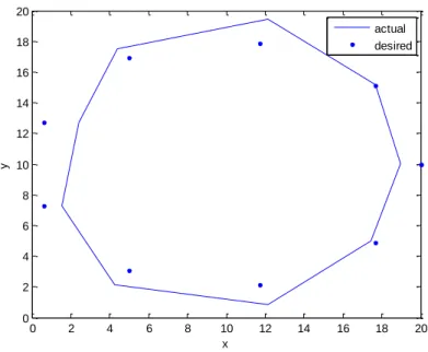
Fig. (4.2) (six target points and the obtained torque curve). 2) Generation of ten point paths and 19 design variables without prescribed timing: design variables are. The time taken to run the program in MATLAB was 10.09 seconds to display the results as below. The time taken to run the program in MATLAB was 10.97 seconds to display the results as below.
The time taken to run the program in MATLAB was 04.17 seconds to show the results as below. Current points which are tracked by the connecting link and precision points case 2(2) SL. The objective function i.e. path error varies with respect to the number of precision points specified.
Comparison With Genetic Algorithm
Path Synthesis Without Prescribed Time
For the first problem, a program written in Matlab consisting of three files, namely hmsc1, feasble1 and pathec1, was created for path synthesis without prescribed time.
CONCLUSIONS
Future Scope Of The Work
Also as in hybrid synthesis approach, the same coupling can be adopted for both path synthesis applications as well as motion synthesis applications. Matlab programs for four cases considered in the work are based on the following flowchart.