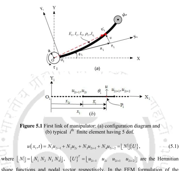
89 Figure 5.2 (a) Diagram of the configuration of the second link of the manipulator, and. b) Typical j-th finite element of the second bond with 8 dof. 91 Figure 5.3 Typical results: (a) Center angle (shoulder) and (b) residual vibration. c) residual vibration (type1), (d) residual vibration (type2).
Flexible Manipulators …
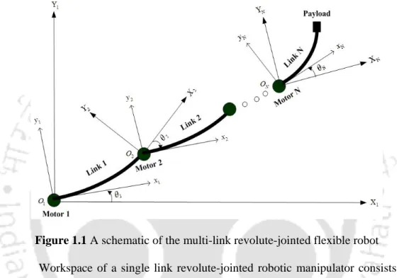
The working area of a single-joint revolute-jointed robot manipulator consists of the points on the circumference of the circle. Some of the applications of single link flexible manipulator are waste tank cleaning, operating microsurgical applications, deburring, surface polishing, grinding, etc. [Hakki, et al., 2012].
Motivation
Problem Statement
Organization
Dynamic modeling and shape optimization of rigid-flexible manipulator and double-joint flexible manipulator as opposed to single-joint manipulator are presented in chapter 4 and chapter 5 respectively. Shape optimization is performed in all cases of flexible manipulators using classical optimization technique - sequential quadratic programming (SQP).
Conclusion
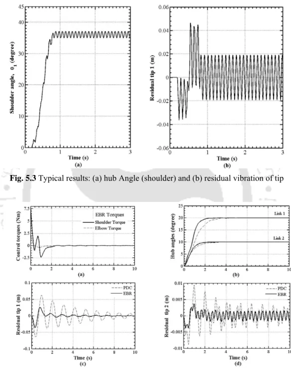
The comparative dynamic response of the single-link flexible manipulator is performed for different torque excitation profiles. Vibration suppression of the single/double link flexible manipulator is also presented under energy-based controlled torque (EBR) excitation.
Introduction …
Dynamic Modeling
Finite Element Based Modeling
- FEM Modeling of Single Link Flexible Manipulator
- FEM Modeling of Multi Link Flexible Manipulator
The finite element method requires transformation of the governing differential equation into a suitable integral equation. Simulated results indicate that dynamic behavior of the flexible double joint manipulator is highly non-linear and complex in nature.
Assumed Mode Method Based Modeling
- Modeling of Single Link Flexible Manipulator
- Modeling of Double Link Flexible Manipulator
The asymptotic perturbation method is an effective tool for analyzing the distributed parameter model of flexible manipulator. Lagrangian adopted mode method incorporating the measured linear displacements and angular deflection of flexible links is used to derive the dynamic model of the flexible manipulator.
Experimental Observation
1997] performed experiments for two-degree-of-freedom single-link flexible manipulator with hydraulic actuator. Milford and Asokanthan [1999] derived exact partial differential governing equations for system states of two-link flexible manipulator.
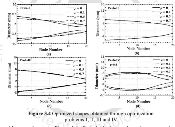
Shape Optimization
Structural Optimization
All the structural optimization studies discussed above were devoted to the beams rigidly attached to an inertial frame. Also, the bottom of the flexible link must be rigidly attached to the rotating hub for mechanical support.
Optimum Shape Design of Flexible Manipulators
Finite element method and assumed state method have been widely used for dynamic analysis of flexible robot manipulator. However, not much research has been done on shape optimization of flexible robot manipulators.
Challenging Issues
Maximizing higher natural frequencies through shape optimization provides higher frequency bandwidth for the operation of the flexible robotic system. Optimizing the shape of the links for a specific payload may not improve the dynamic response at higher payloads.
Introduction
Mathematical Modeling
Computation of Kinetic Energy of the Link Element
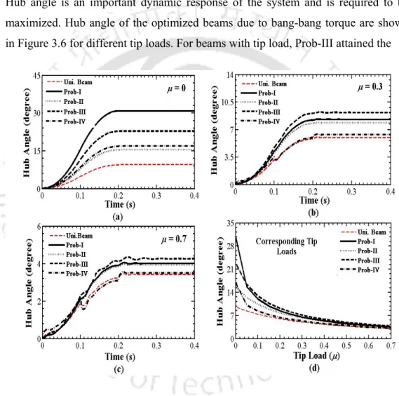
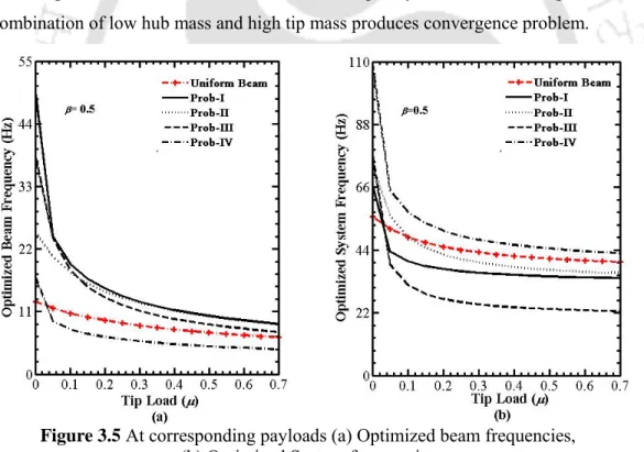
The hub angle of the optimized supports due to the pop-pop torque is shown in Figure 3.6 for different tip loads. The improved fundamental frequency of the optimized link (Prob-II) with respect to the single link is shown in Figure 3.33. Optimization problem-II (maximization of fundamental link frequencies under its mass constraints) yields overall improved system dynamics.
Computation of Potential Energy of the Link Element
Lagrange's Equation of Motion in Discretized Form
The kinetic energy and potential energy of a system are obtained by calculating the energy of each element of the system and then adding all the elements together. The Lagrange system is given by L T V= − and then the Lagrange equations of motion of this dynamical system can be written as The effects of hub inertia and payload mass are incorporated into the global mass and stiffness matrix using the Dirac-delta function as described by Dixit et al. 3.19) becomes a standard eigenvalue problem and is solved for the eigenfrequencies of the system.
Boundary Conditions
Natural Boundary Conditions
Essential Boundary Conditions
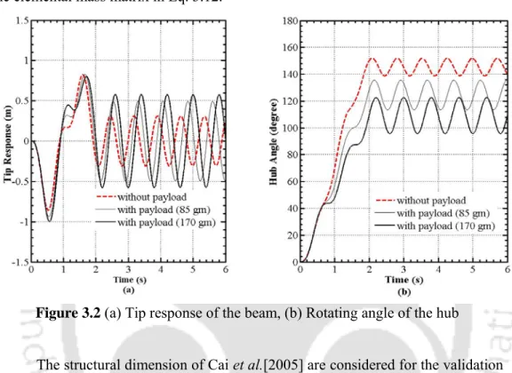
Model Validation
Bathe , 1996 ], where ωmax is the highest beam frequency and ∆tc r denotes the maximum time step consistent with numerical stability. Since the robotic system operates at moderate speeds, the model is linearized by neglecting the nonlinear term (Mnl) of the elemental mass matrix in Eq. 2005] are not shown here to preserve the clarity of the figures. The developed model can be considered for the optimization of the rotary joint shape for four different optimization problems.
Optimization Procedure
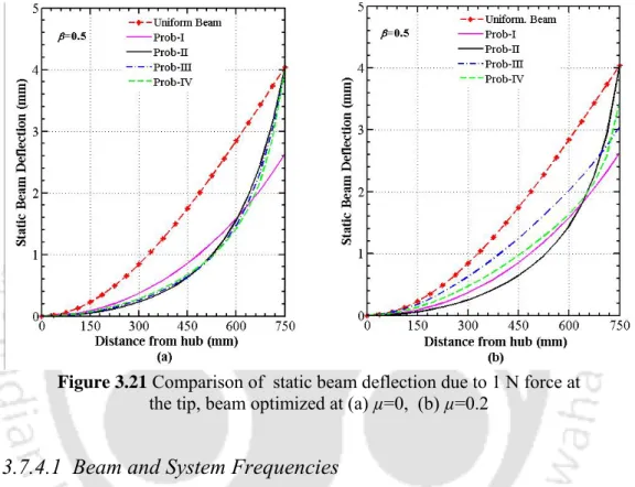
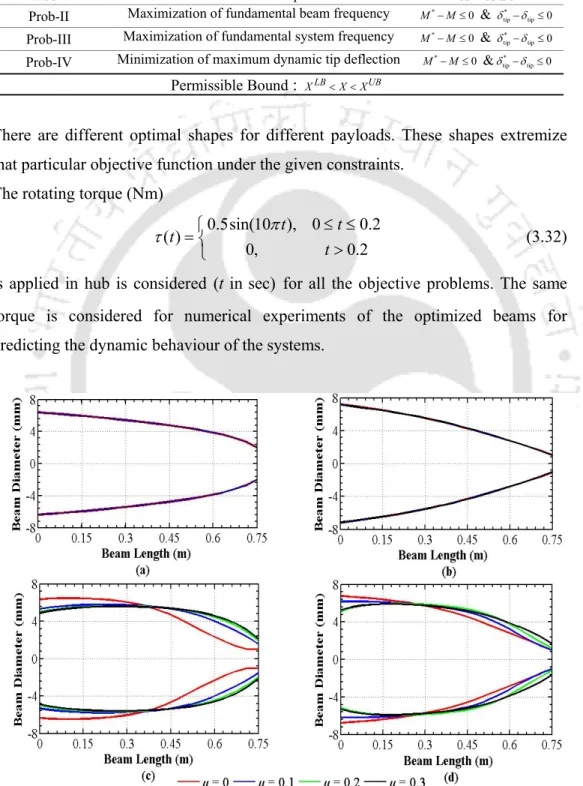
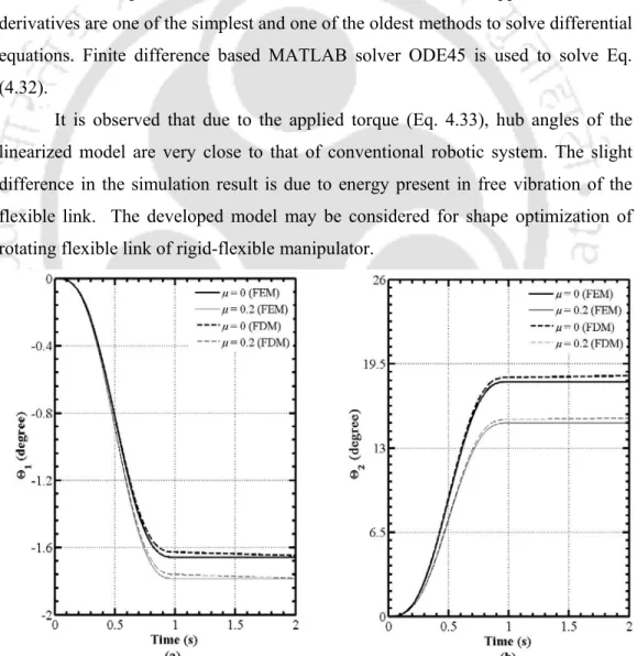
Here the same sinusoidal excitation torque (7sin ) Nmπt is considered for 2 sec about the axis of rotation. It is observed that the linearized model here at very high torque amplitude (7 Nm), peak responses and hub angles is very close to Cai et al. Maximization of the fundamental frequency is considered as a goal for high-speed operation of the robotic system, and minimization of static deflection is considered as a goal for accurate positioning of the robot manipulator.
Results and Discussion
Shape Optimization …
- Beam/system Frequency
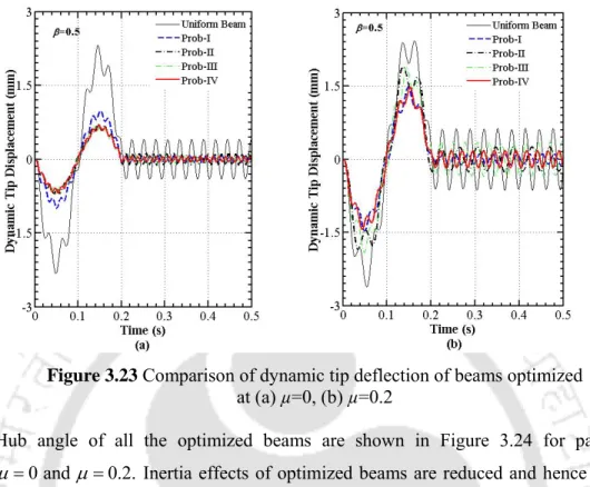
- Hub Angle and Static Tip Deflection
- Dynamic Response
- Comparison of Optimization Problems and Links
Note that the masses of the optimized beams are equal to the mass of the uniform beam (0.1596 kg). Thus, the masses of the optimized carriers are active constraints in a rigid-flexible robotic system. It can be seen that the dynamic response of the system is very sensitive to the set of optimized connections.
Proposed Optimized Shape for Varying Tip Loads
- Comparative Study of Proposed Designed Shapes …
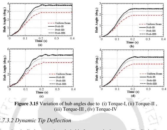
Effect of Different Excitation Torque Profile
- Hub Angle
- Dynamic Tip deflection
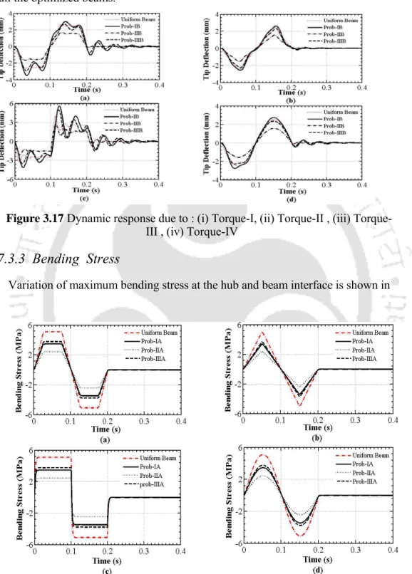
- Bending Stress
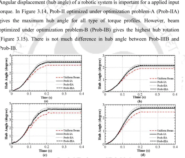
Four different types of input torque are considered as shown in Figure 3.13 to predict the dynamic behavior of the optimized beams. In Figure 3.14, Prob-II optimized under optimization problem-A (Prob-IIA) gives the maximum center angle for all types of torque profiles. Importantly, all optimized beams yield higher central angle than uniform radius in both optimization problems.
Shape Optimization for Vibration Suppression
- Beam and System Frequencies
- Dynamic Response of the System
- Sensitivity Analysis of Active Constraint M *
Optimized forms of the manipulator for the optimization problem defined in Table 4.1 are plotted in Figure 4.3. The dynamic response of the flexible double-link manipulators also depends on the length ratios of the links. In all optimization problems, it is noted that the mass of the optimized links are the active constraints.
Shape Optimization of Higher Natural Frequencies
Improved Dynamics through Controlled Torque
- Optimization Procedure
- Comparative dynamic Study under Controlled Torque 63
K = J + m L + m L f (3.35) The PD controller can stabilize the system, but the vibration of the flexible beam cannot be controlled. For the comparative dynamic response of the flexible robot joint, a sinusoidal torque is applied about the rotation axis for numerical investigation as shown below. In the simulated numerical results, it is observed that the residual vibration of the tip of the uniform joint is enhanced under controlled torque.
Introduction
Since the residual vibrations from flexible manipulators affect the tasks to be performed by the robotic system, the combination of rigid-flexible links is considered for its optimal design.
Modeling and Solution Technique …
Kinetic Energy Computation of the Link Element
The potential energy of the ith element of link due to elastic deformation is given by. Potential energy of the ith element of 1st link due to elastic deformation is given by. Therefore, improved dynamics of the optimized links are sensitive to the increase in link masses.
Elastic Potential Energy Computation of the Link Element
Lagrange's Equation of Motion in Discretized Form
Effects of Hub, Rigid Link, Motor Mass and Payload Inertia
Boundary Conditions
Natural Boundary Conditions
Natural boundary conditions are applied at the second joint of the manipulator system, i.e. component of the shear force at the end point of the first link( )F1 must be balanced by the shear force at the same node to the second link (F2, 1) of the manipulator given by. F +F θ = (4.25) Torque at the first load is added by the reactive torque on first link (rigid) through the second link is given by. 4.26) Other forced boundary conditions, bending moment and shear force at the end of second link are zero are as given by.
Essential Boundary Conditions
Optimization Procedure
Results and Discussion
- Model Validation
- Shape Optimization and Static Tip Deflection
- Beam and System Frequencies
- Dynamic response of the System
- Active Constraint M *
Fundamental beam and system resonance frequencies of the optimized beams at µ=0 and µ=0.2 for selective payloads are plotted in Figures 4.5 and 4.6. Dynamic responses of the optimized beams under different optimization problems are shown numerically in tabular form (Table 4.3). It is observed that masses of the optimized flexible beams are equal to the mass of uniform beam (0.1596 kg).
Summary
Introduction
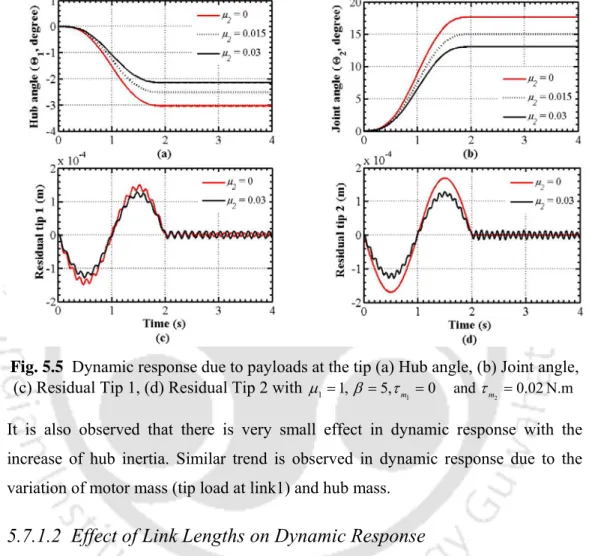
The dynamic behavior of the flexible double link manipulator changes with respect to the change of charge at the end of the second link, as shown in Figure 5.5. The mass of the optimized links is less than or equal to the mass of the individual links. By increasing the mass of the optimized links (10%), the robot system is observed to move towards the rigid system.
Liao, Y.S., (1993), A generalized method for the optimal design of beams under flexural vibration, Journal of Sound and Vibration, 167(2), s. 1988), A Lagrangian formulering af den dynamiske model for fleksible manipulatorsystemer, ASME Journal Dynamic System, Measurement and Control, 110, s. Rakhsha, F., og Goldenberg, A.A., (1985), Dynamic modeling of a single link fleksibel robot, Proceedings of the IEEE International Confrence on Robotics and Automation, pp.
Obtaining Elemental Equation of Motion of Manipulator …
Modeling of the First Link
- Kinetic Energy of the i th Element of the 1 st Link …
Modeling of the Second Link
- Kinetic Energy of the j th Element of the 2 st Link ….…. 92
Boundary Conditions
Natural Boundary Conditions
The natural boundary condition is applied to the second joint of the manipulator system, i.e. component of the shear force at the end point of the first member. F n− ) must be balanced by the shear force at the same node to the second link (F2,1) of the manipulator given by. i) bending moment at the end of the links. ii) shear force at the end of the second member.
Essential Boundary Conditions
Effect of Hub Inertias and Tip Loads
Model Validation
Therefore, the developed model is considered for the optimization of the shape of rolling joints for optimization problems.
Results and Discussion
Parametric study
- Dynamic response due to Different Payloads
- Effects of Link Lengths on Dynamic Response
- Dynamic Response due to Different Input Torques…
- Comparative Dynamic Response due to Different
- Dynamic Response due to Payloads
- Optimization Procedure
- Optimized Dynamic Response …
- Optimized Links under Controlled Torque Excitations
- Effect of Active Constraint M * …
It is observed that there is a decrease in the hub angle and an increase in the joint angle with the increase in the torque amplitude. From Figure 5.20, it can be seen that residual vibrations of the optimized links are further suppressed in the case of control torque excitations compared to bang-bang torques. It is observed that the mass of the optimized beams is equal to the mass of uniform joints (0.2128 kg and 0.1703 kg, respectively) and it is therefore an active constraint.
Summary
Conclusions …
There are further variations of the optimized forms for different payloads in almost all optimization problems. In all the optimization problems, lots of links are redistributed towards the root of the individual links. Shape-optimized links for one target may perform even worse in other targets than in the case of the uniform links.
Scope of Future Work
Baruh, H., and Tadikonda, S.S.K., (1989), Dynamics and control issues of flexible robotic manipulators, AIAA Journal of Guidance, Control and Dynamics, 12(5), p. 1989), Timoshenko vs. Bernoulli-Euler beam theories for inverse dynamics of flexible robots, International Journal of Robotics and Automation, 4(1), p. Farid, M., and Lukaiewicz, S.A., (2000), Dynamic modeling of spatial manipulators with flexible links and joints, Computers and Structures , 75, p. 1985), Flexibility control of elastic robotic arms, Journal of Robotic Systems, 2(1), p. 1987), Modeling and control characteristics for a two-degree-of-freedom coupling system of flexible robotic arms, JSME, Series C, 30, p. Naganathan, G. and Soni, A.H., (1988) Nonlinear modeling of kinematic and flexible effects in manipulator design, ASME Journal of Mechanisms, Transmissions and Automation in Design, 110, p. 1987) , Coupling effects of kinematics and flexibility in manipulators, The International.