MR image at varying noise levels. a) RMSE versus the noise level σn (b) SSIM versus the noise level σn (c) Contrast versus the noise level σn. 114 6.8 Comparative plot of denoising results obtained for the simulated T2-weighted axial MRI. image at varying noise levels. a) RMSE versus the noise level σn (b) SSIM versus the noise level σn(c) BC value versus the noise level σn (d) Contrast versus the noise level σn.
Denoising in Magnetic Resonance Imaging
Motivation for the Present Work
Therefore, if the wavelet filters are modified to adapt to the local spatial activity around a pixel as in nonlinear filters, it can be expected to have better feature preserving ability. The proposed work links the local spatial interaction with the wavelet features to result in good feature-preserving denoising.
Contributions of the Thesis
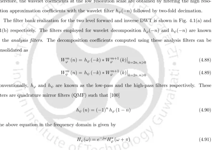
Therefore, this work opts for a nondecimated wavelet transform that reduces the technique to redundant subband decomposition. Therefore, our research is motivated to develop a UDWT-based denoising framework that uses bilateral filtering to exploit the intra-scale dependencies of the scaling and the wavelet coefficients.
Organization of the Thesis
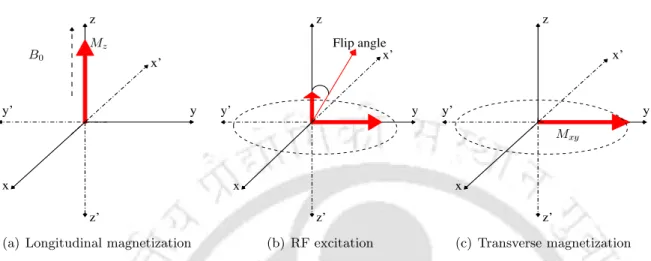
Magnetization phenomenon
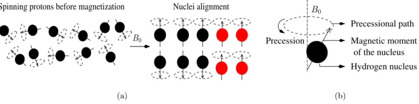
- Nuclei alignment
- RF excitation
- T1 relaxation
- T2 decay
Under the influence of a strong external magnetic field (B0), slightly more protons align parallel to B0 and cause longitudinal magnetization. b) precession of the hydrogen nucleus along the B0 direction. As a result, the nuclei emit the absorbed energy and the orientation of the spins is re-established parallel to B0.
Pulse sequence mechanisms
- Spin echo sequence
- Gradient echo sequence
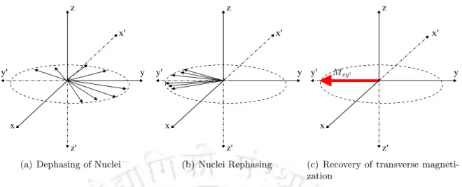
To produce images from the transverse magnetization, additional pulse sequences are therefore applied to rephase the spins and compensate for inhomogeneities of the magnetic field [21]. During the relaxation process Mxy. b) T2 is the time it takes for the spins to dephase in the transverse plane, causing the transverse magnetization to return to its equilibrium value, zero.
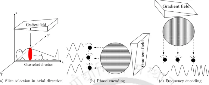
Spatial encoding using gradients
- Slice selection
- Phase and frequency localization
- k-space encoding
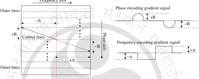
If the gradient of the phase encoding is positive, the upper half of k-space is encoded. A and +B are positive amplitudes (−Aand−B are negative amplitudes) of the phase and frequency encoding gradient signals respectively.
MR Image Characteristics
- Contrast
- Spatial resolution
- Signal-to-noise ratio
- Field strength
- Coil type
- TR
- TE
- Flip angle
- Significance of SNR and its trade-offs
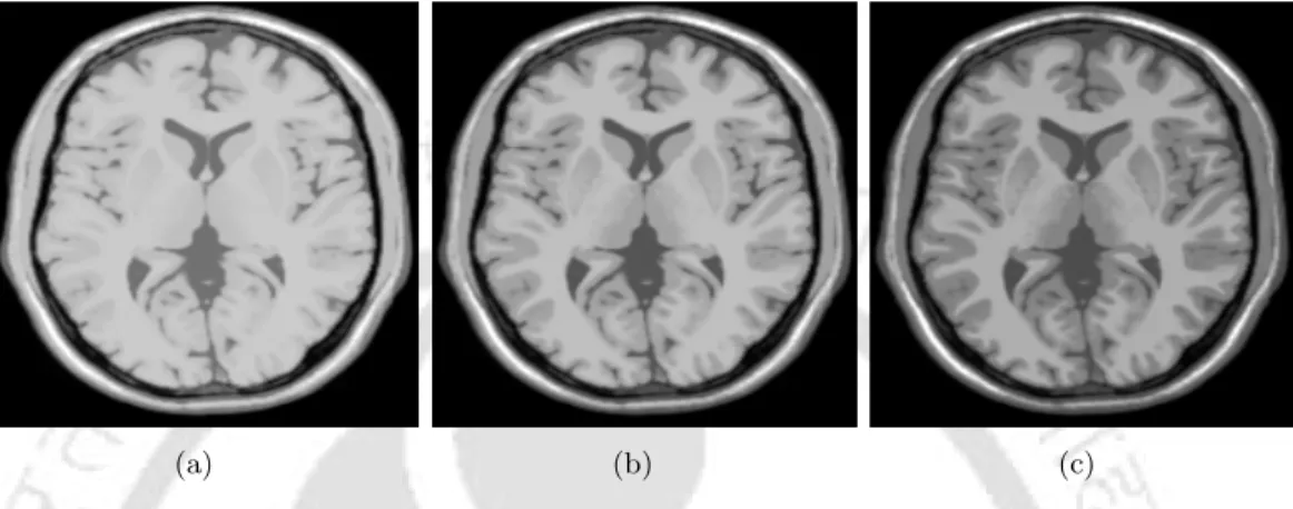
Details on T1 and T2 weighted images for different values of TR and TE are illustrated through Figs. Tissue boundaries are very distinct on T1-weighted images and are therefore particularly used to study anatomical details.
Summary
However, calculating the size of the complex MR image changes the intensity distribution of the size data. The characteristics of the noisy MR image are also affected by the number of RF coils used for acquisition.
Characteristics of Noisy MR image
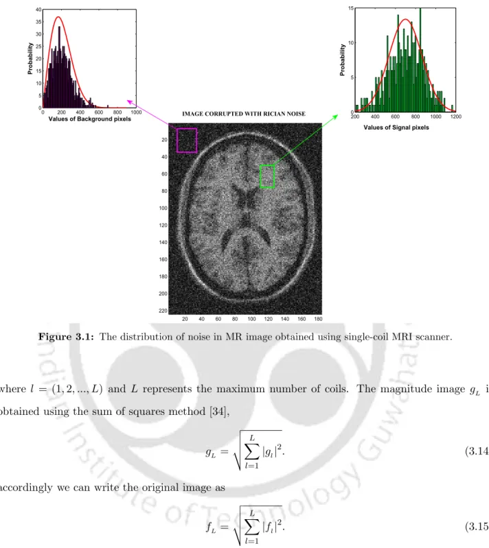
Characteristics of noise in single coil system
Similar to size image, the phase MR image is also obtained by non-linear operation. Since the arctangent operation is a nonlinear function, the distribution of phase MR image also tends to be Rician [ 29 , 33 ].
Characteristics of noise in multi-coil system
This distribution function does not give the distribution of noise in the image, it gives the distribution of the observed pixel intensities in the presence of noise [32]. n is zero, the Rician pdf given in Eq. 3.9) leads to Rayleigh scattering and it is defined as follows. The image regions with large signal intensity approximate Gaussian pdf [29]. and the distribution function is given by.
Noise Variance Estimation
Thus by considering E[g2] as the average value µ calculated from a portion of the background region, the noise standard deviation is estimated as. In all our denoising methods presented hereafter, the noise variance is estimated from the background regions of the MR image using equation Eq.
Summary
In this chapter, we discuss the existing state-of-the-art methods for denoising MR images. The extensive literature on MR image denoising algorithms can be broadly classified into spatial domain and wavelet domain methods.
Basics of Spatial Filtering
Popularity of wavelet domain methods in denoising applications is mainly due to the energy compaction property [5] of the wavelet transform. The filter weights used in spatial filtering approaches are independent of the content of the image.
Spatial Filtering Techniques for MRI Denoising
- Gaussian filtering
- Measurement dependent filtering
- PDE based denoising
- Neighborhood based filtering
- Bayesian denoising
- Wiener filtering
- AVREC based filtering
- Non-local means filtering
The idea behind this filter is to embed the original image in a family of derived images f(x, y, σ), obtained by convolving the original image f0(x, y) with a Gaussian kernel G(x, y, σ) of variance σ2, expressed as. 4.9) The family of derivative images can be represented as a solution of the heat diffusion equation. In this method [59], the matrix expansion is based on the statistical properties of the local structures in the image.
Theory of Wavelet Transform
- Wavelets and wavelet transform
- Wavelets as filters
- Formulation of Discrete Wavelet Transform
- Scaling functions
- Wavelet functions
- Wavelet series expansions
- Discrete wavelet transform
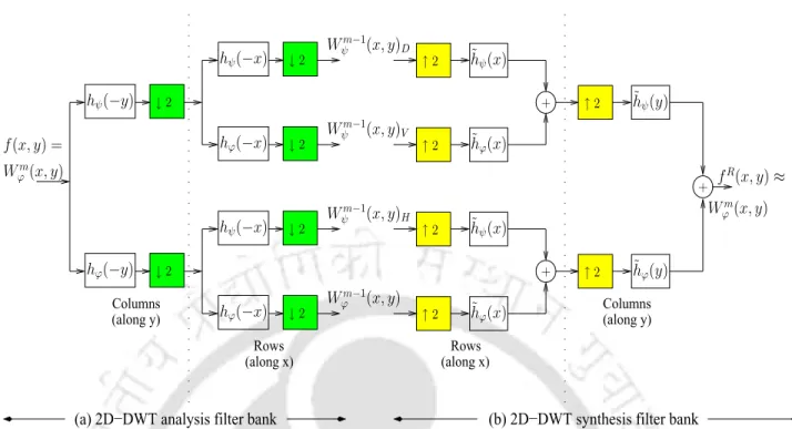
- Filter bank implementation of DWT
- Two dimensional DWT
- Modifications of DWT
Using the orthogonality of the wavelet bases, the inverse continuous wavelet transform is calculated as. Therefore, the ripple function at scale m can be expressed in terms of the scale function at scale m+ 1 axis.
Wavelet based MRI denoising
The proposed method tends to effectively reduce the noise in the background (no signal) region of the image. The value of K was determined to be equal to two for MR images in terms of SNR.
Summary
The aim of this chapter is to present the proposed waltz domain bilateral filter (WD-BF) strategy and to validate its applicability for denoising MR images. The proposed technique is validated by comparing the denoising results of the WD-BF representation with other existing wavelet decompositions, which include DWT and conduction invariant wavelet transform.
Translation Invariant Wavelet Decompositions
Stationary wavelet transform
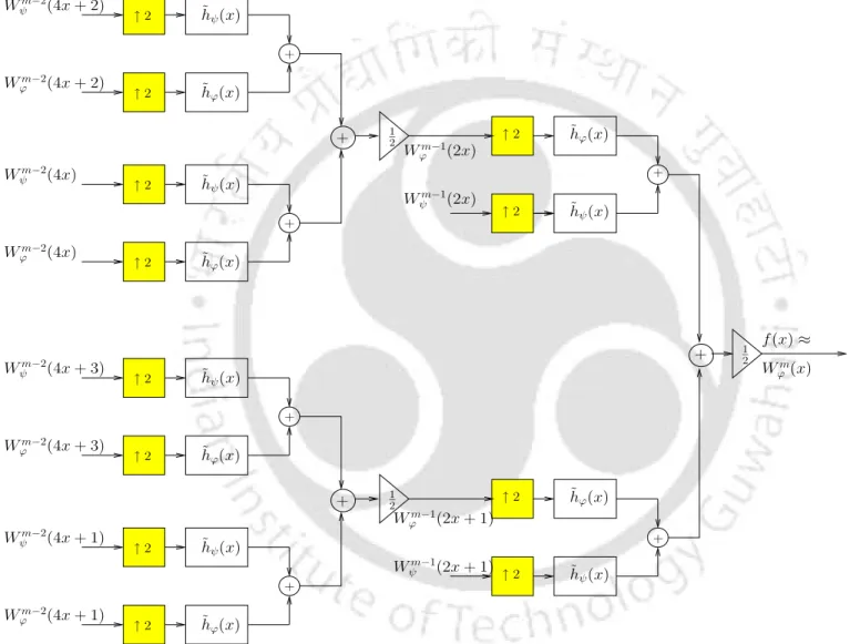
The multi-resolution property is preserved by upsampling the hϕ and hψ filters at each scale by a factor of 2J−1−m. Upsampling in the time domain reduces the bandwidth of the filters by a factor of two between successive levels of resolution.
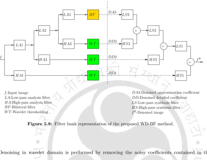
Proposed wavelet domain bilateral filter
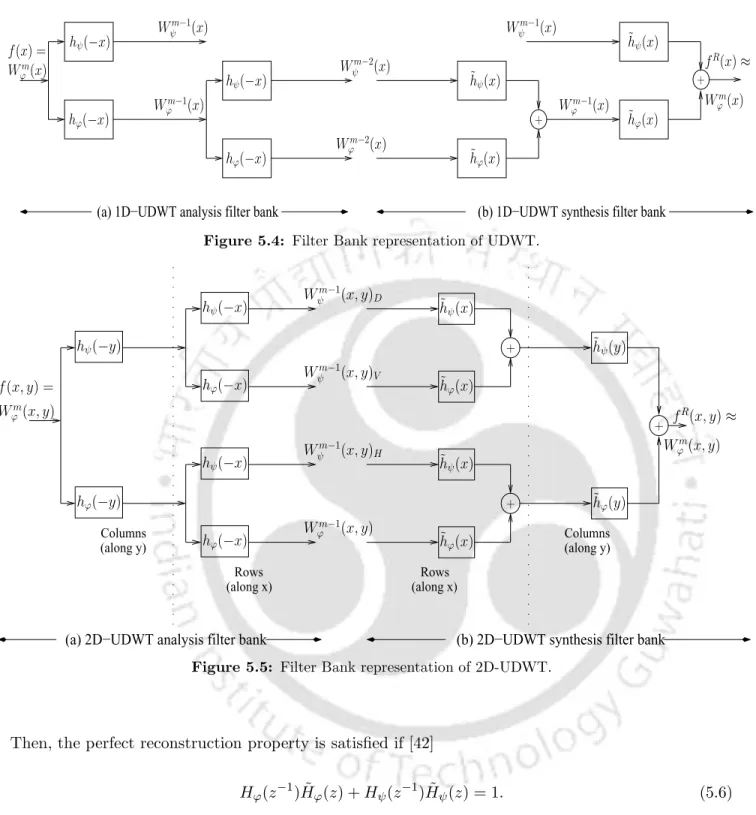
- Undecimated wavelet transform
- Bilateral filter
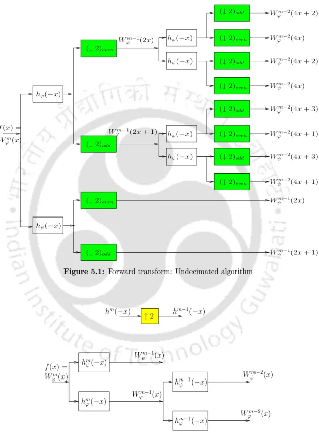
The system input f(x) is decomposed into the approximation coefficient Wϕm(x) and the detail coefficient Wψm(x) at each levelm. However, the bilateral filter parameters can be optimized when the noise characteristics are well understood.
Wavelet Thresholding
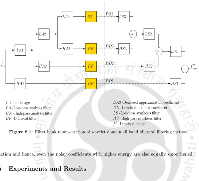
Since the noise characteristics can be studied from the detail wave coefficients, the performance of the bilateral filter in the wave domain can be optimized. The schematic representation of the WD-BF applying the wavelet threshold approach for denoising MR images is given in Fig.
Bias Removal in MR images
It also reduces the tissue contrast of the MR image as the noise level increases. Therefore, as stated in [37] the bias in the square magnitude domain is constant and is independent of the signal intensity.
Validation of WD-BF for MRI Denoising
Validation strategies
SSIM is the effective alternative that improvises the error measurements and is also consistent with the visual perception. The final value of SSIM is the average of the SSIM index calculated over the local R regions.
Experiments and results
- About the dataset
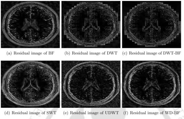
- Comparative evaluation
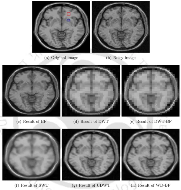
The denoising results of the T1-weighted simulated MR image corrupted by 5% noise are shown in Figure. The evaluations of the noise reduction methods on the T2-weighted simulated MR image for different noise levels are shown in Figure 2.
Summary
The corresponding values of the quality metrics that validate the denoising results are given in Table-5.4. The next chapter presents an adaptation of the NeighShrink threshold in the WD-BF framework and experimental evaluation for the optimal choice of bilateral filter parameters.
NeighShrink Wavelet Thresholding
The optimal values of the filter parameters are suggested by performing experiments on a sufficiently large number of MR images at varying noise levels. The discussion of the experiments and results are presented to validate the effectiveness of the improved WD-BF technique for feature-preserved MR image decomposition.
Influence of Bilateral Filter Parameters
Effect of R neigh
E{SU RE(wm, λ, L)} (6.9) Accordingly, the optimal threshold λ and the size of the adjacent window Lm for the subband m that minimize SU RE(wm, λ, L) are chosen.
Effect of σ d
Effect of σ r
Experiments and Results
Parameter selection
- Choice of R neigh
- Choice of σ d and σ r
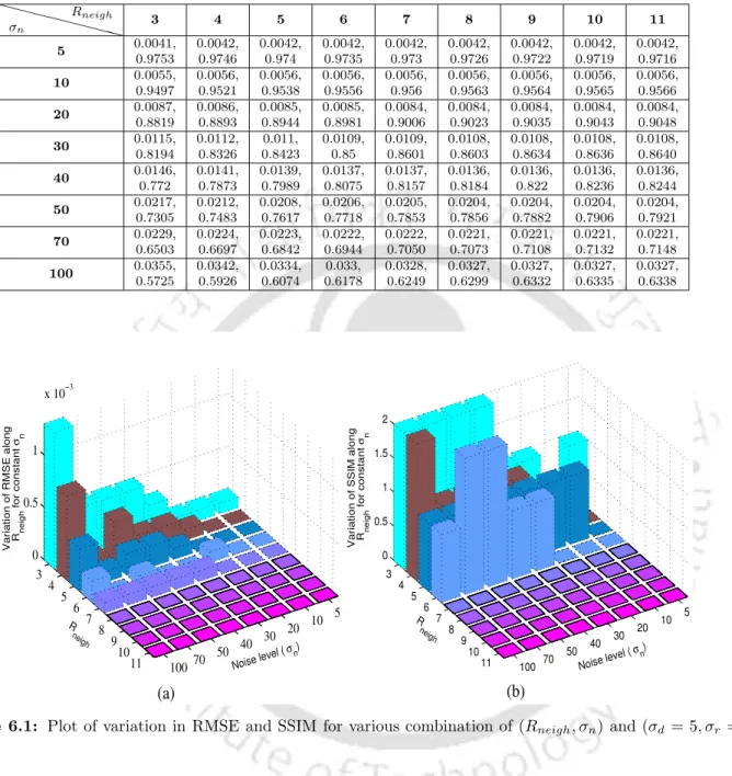
It gives the average RMSE and SSIM values obtained for different choices of Rneigh and σn. The optimal range of RMSE and SSIM with respect to σr is around 0.9σ to 1.9σna and for σd ≥5 for all noise levels.
Denoising results - A comparative validation
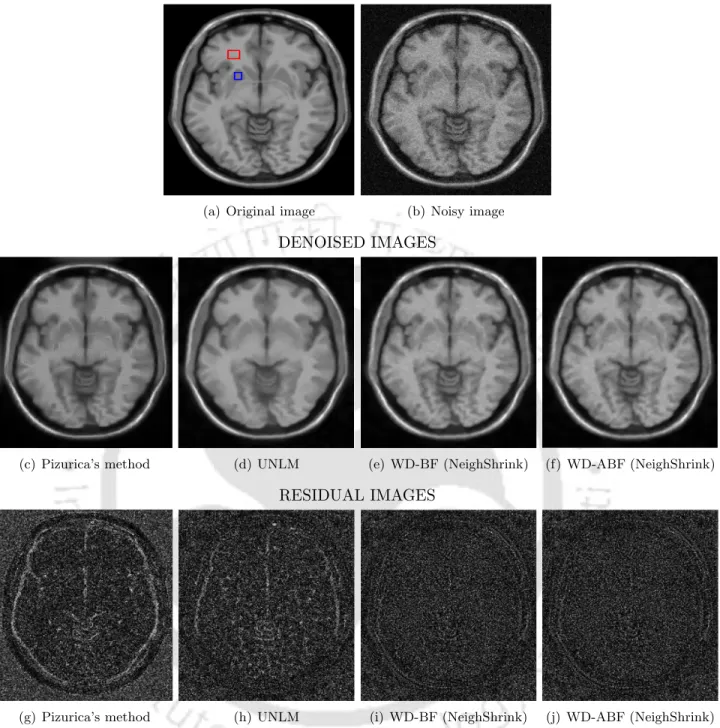
- Evaluation on simulated dataset
- Evaluation on clinical dataset
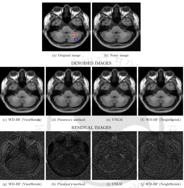
At lower noise levels, the UNLM approach is better than the WD-BF (VisuShrink) method. At low noise levels, the performance of Pizurica's method and UNLM is better than WD-BF (VisuShrink).
Summary
Also, the contrast of the attenuated MR image is very poor for higher noise levels. But this adjustment of bilateral filter in most of the experiments did not produce very significant improvement in the WD-BF framework.
Automatic Parameter Selection
The 2D maps illustrate the pixel-wise σr values obtained with respect to the standard deviation σxy of the pixel. The 2D maps illustrate the pixel viseσr values obtained with respect to the standard deviationσxy of the pixel.
Results and Discussion
The comparative graphs of denoising results obtained for different noise levels are given in Fig. The graphs of denoising results obtained for different noise levels are given in Fig.
Summary
Accordingly, we proposed two basic approaches based on a bilateral filter to reduce the noise of detail coefficients. With these basics, the proposed adaptive VisuShrink and double-sided filter-based waltz denoising are explained.
Wavelet Thresholding Approaches
Thresholding rules
- Hard thresholding
- Soft thresholding
- Neighblock thresholding
Wavelet thresholding is a nonlinear technique that removes or reduces the wavelet coefficients based on a threshold. The size of the wavelet coefficients corresponding to the noise pixels is smaller than the signal coefficients.
Threshold selection
- Universal threshold
- SURE threshold
- Bayes threshold
For a known noise variance σ2n, the value of σθm is given by σθm =. 8.12) Therefore, the subband Bayes threshold is formulated as follows. The thresholdλbayesminimizes the Bayesian risk estimate defined as. 8.14) where ˆθm is the estimate of θm obtained by soft thresholding.
Adaptive VisuShrink - Proposed method
With this motivation, we proposed a simple modification of the universal threshold by including the spatial context information. The universal threshold as in Eq. 8.5) shows that the threshold is proportional to the data length.
Bilateral Filtering as an Alternative to Wavelet Thresholding
The important parameter that determines the extent of smoothing in the bilateral filter is the width of the range kernel σr. Therefore, the width of the range filter depends on the level by choosing it as.
Experiments and Results
Evaluation of adaptive VisuShrink
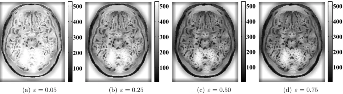
- Choice of ε and neighborhood
- Denoising results
Thus the eλadap value becomes large and results in excessive smoothing of structural details as in VisuShrink. However, due to limits on the smoothing measure, some of the noise coefficients remain unfiltered.
Evaluation of bilateral filtering over wavelet thresholding
- Parameter selection
- Denoising results
Summary
Suggestions for Future Research
Introduction
The first method is called Adaptive VisuShrink and is designed by changing the universal threshold based on the spatial context of the wavelet coefficients. The basic idea in adaptive VisuShrink is to limit the universal threshold based on the spatial support of the wavelet coefficient to be removed.