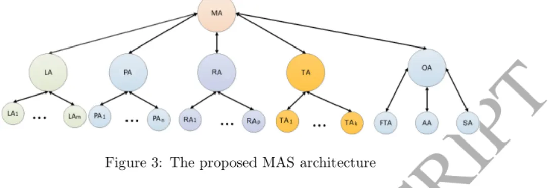
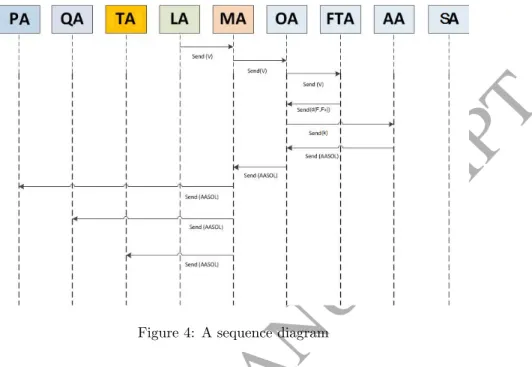
The MAS we refer to here is structured in different types of agents that manage the characteristic elements of the grid (e.g. load demand, power generation, active power) and the OPF problem. In the online phase, appropriate agents first apply the F transformation to the vector of the measured smart grid state and determine the reference cluster. In Chapter 3, the theoretical foundations and main features of the proposed framework are presented.
The vector of state variables x in it can be represented by several quantities, such as the magnitude of the voltage on the load buses and the reactive power output of the generators. Similarly, the control variable vector u can be written primarily in terms of some quantity, such as the active power output of the generators and the magnitude of the voltage at the generator buses. The power flow problem can be stated as a special instance of the OPF problem (see [31] for details).
IPM appears to be one of the most efficient algorithms for solving the OPF problem [22, 45]. In the resulting algorithm, each agent represents an individual in DE, which is a solution vector of the OPF with its fitness value. Three test cases were examined, exhibiting an increasing computational time with the grid dimension.
In the context of SG, it is common to mention big data due to the ever-increasing historical data [11].
ACCEPTED MANUSCRIPT
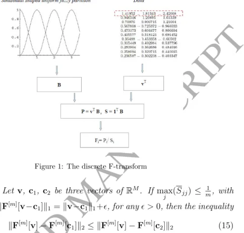
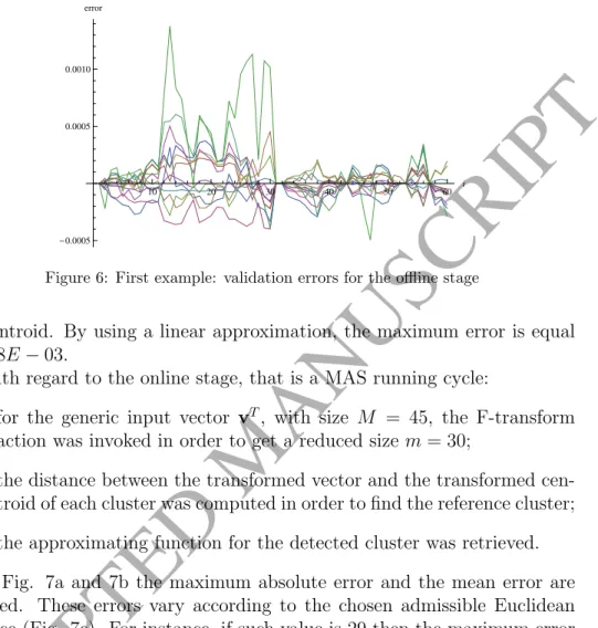
DF =AF[nm]BT, (12) for the two-dimensional case, being F[nm] the matrix obtained by Eq. As a reminder of this work, k(.)kp will denote the p–norm and IN will denote the identity matrix of order N. The offline stage is firstly aimed at compressing the historical data in order to respond to storage saving issues and secondly at finding the approximate relationships between some measurements and the optimal settings of the problem defined in Section 2.
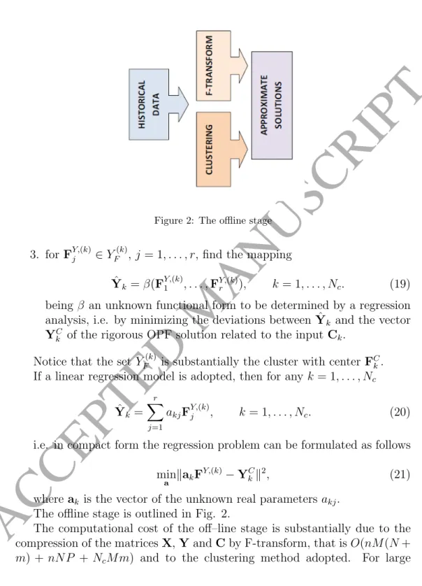
The rows of X are the state vectors of the power system vTj = (xj1, ..., xjM), here including the active and reactive powers measured on each network bus, while the rows of Y are the vectors of the corresponding OPF solutions. Let C be an Nc×M matrix, whose rows are the vectorsCk representing mainly the centers of the Nc clusters, and let YC be the Nc×P matrix, whose rows are the vectorsYCk of the rigorous OPF solution related to the inputCk. The computational cost of the offline phase is largely due to the compression of the matrices X, Y and C by F transformation, i.e. O(nM(N+ m) +nNP + NcM m) and to the clustering method used.
The online stage is referred to the monitoring of the network, by calculating the optimal setting through the OPF solution for the online measurements. The usual requirements regarding scalability, reliability, resource optimization and soft real-time modeling are pursued by allowing for the dynamics of agents on a network of computers, which as a unique constraint requires the presence of the plug-in DICE component on the machine. Matpower is based on IPM, which is one of the most effective methods for solving OPF problems, as mentioned in Section 2.
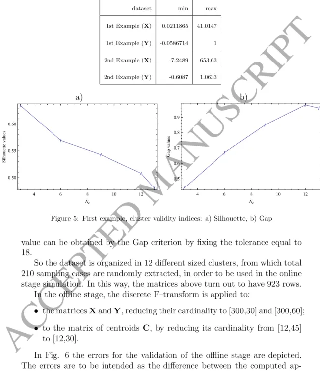
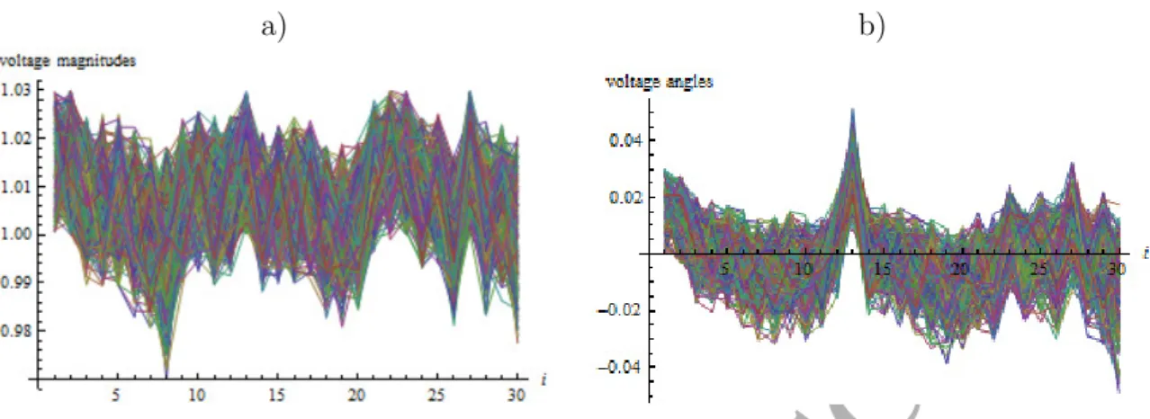
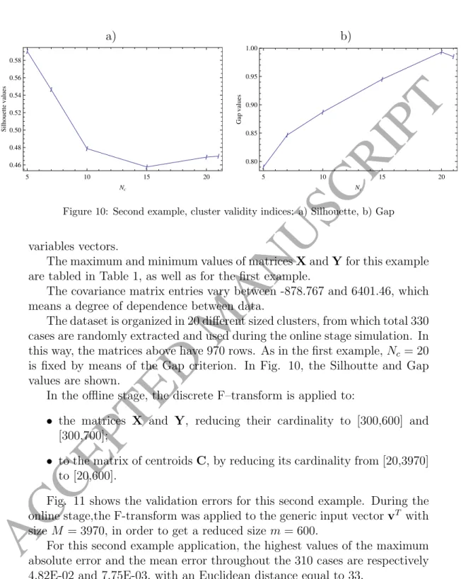
The first example application covers the solution of the OPF problem for the IEEE 30 bus test system. The data set is composed of a 1133 x 45 matrix (X matrix) of values of input state variables (that is, the values of 45 state variables, in terms of active and reactive power in 1133 moments) and a 1133 x 60 matrix (Y matrix), whose rows represent the OPF solutions (that is, bus voltage magnitudes and angles) for the corresponding vector of 45 state variables. The covariance matrix of the entire data set shows some degree of dependence as the values vary between -9.775 and 27.749.
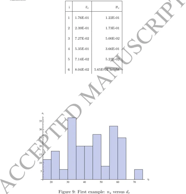
The mean error ec and the standard deviation σc affecting the ith control variable (in p.u.) are shown in table 2. These results are good enough, considering that the maximum values of mean error and standard deviation for the pre-. For about 1/3 of the sample cases, the running time for the calculation of the exact solution is 50−60% higher than the one for the calculation of the approximate solution; for about one half of the sample cases, the running time for computing the exact solution is 30-50% higher than the one for computing the approximate solution. In order to further test the performance of the proposed methodology, the constrained power flow analysis of the 2383-bus Polish power system, representing the Polish 400, 220 and 110 kV networks consisting of 2383 buses, 327 generators, 2056 loads and 2896 lines, were considered.
The maximum and minimum values of the XandY matrices for this example are shown in Table 1, as well as for the first example. For this second application example, the highest values of maximum absolute error and mean error across 310 cases are 4.82E-02 and 7.75E-03, respectively, with a Euclidean distance equal to 33. For 2/3 of the sample in cases , the execution time for computing the rigorous solution is 35−55% higher than that for computing the approximate solution; for about 1/6 of the sampling cases, the execution time for computing the rigorous solution is 60−80% higher than that for computing the approximate solution.
Numerical results, supported by some theoretical achievements, were obtained for both small and large systems, and they showed the effectiveness of the method.