It is certified that Cheo Jia jun (ID No: 18ACB05681 ) has completed this final year project/dissertation/thesis* entitled “Development of Neural Network Dengue Forecasting Model” under the supervision of Dr. I declare that this report titled “Development of Dengue Forecasting Model with Neural Network” is my own work, except as mentioned in the references.
Introduction
- Problem Statement and motivation
- Project objective
- Project Scope
- C ontribution
- Report Organization
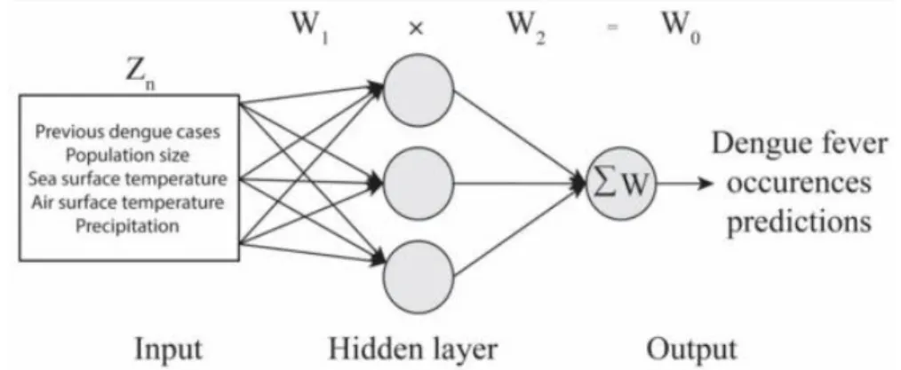
The second objective of this project is to develop a neural network model to predict the number of dengue incidence in Malaysia. The expected output of this project is a prediction model of dengue fever infections among Malaysians.
Literature Review
Review of the Technologies
- Generalized Additive Models (GAMs)
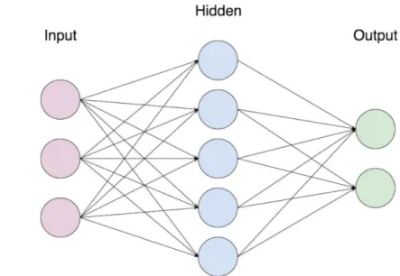
- Artificial Neural Network (ANN)
- Data Collection
- Jupyter Notebook
- Python
- Budget
- Libraries of Python
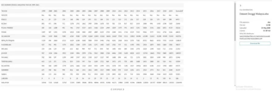
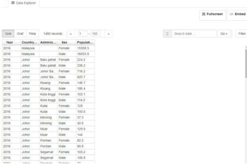
The population is also one of the important factors that can significantly affect the dengue outbreak. The Matplotlib is one of the library of Python used to generate a static, animated and interactive visualization.
Review of the Existing System
- Machine learning and dengue forecasting: Comparing random forests and artificial
- Prediction of Dengue Outbreaks Based on Disease Surveillance and Meteorological
- Superensemble forecasts of dengue outbreaks
- Artificial Intelligence Model as Predictor As Predictor For Dengue Outbreak
- Prediction of Dengue Incidence in the Northeast Malaysia Based on Weather
- Prediction of dengue outbreaks based on disease surveillance, meteorological
This project presents a machine learning-based methodology capable of providing predictive estimates of dengue forecasting in districts of Thailand using data from various data sources. However, these data cannot represent the entire Internet data because Baidu Search Index provides dimensionless data and the website does not provide a specific calculation method, indicating that these data only partially reflect the trend of dengue cases (Liu et al., 2019). However, the lack of online applications that allow authorities to predict the reasonable expected time of the number of dengue cases and determine the forecast of the impact of variables.
This project develops multiple machine learning models to predict the dengue outbreak in Selangor, Malaysia and find the best machine learning model to predict dengue outbreaks. The factors that can influence the outbreak of dengue use in the project are temperature, wind speed, humidity and rainfall. However, the forecast period of this project is very short, which is only 1 month and the result is only available within 400 meters radius, which means that it does not have enough time for the officers in charge of the forecast area to make the strategic preparations to prevent the dengue outbreak, which is contrary to the original intention of giving early warning of dengue outbreaks and because the results are only available within 400 meters, the officers in charge of the forecast area have to spend a lot of time analyzing the facts. (Sundram et al., 2019).
This project develops a generalized additive model (GAM) to predict dengue incidence in Northeast Malaysia with accurate climate data from Kota Bharu Station. Although this project is using GAM as a prediction model, but this project by omitting one of the important characteristics which is population as no population will cause the prediction cannot show how many people suffer from dengue and do not know if dengue level is archived. explosion. The proposal of this project is to develop a system that is able to use the factors that cause dengue outbreak and use it to predict dengue outbreak.
System Model
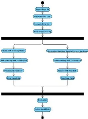
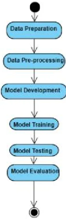
Methodology
Formula
- Formula of Artificial Neural Network
- Formula of Linear Generalize Additive Model
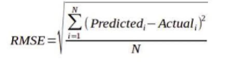
- Formula of Root Mean Squared Error
- Formula of Mean Absolute Error
- Formula of R-squared
In the final stage, we will compare the results generated by ANN and GAM to select the best model as the main prediction model. The linear generalized additive model is used to solve the regression problem, the formula of which is similar to the formula of the linear regression model. Figure 19 shows the absolute error formula used to know the distance between the forecast and the line of best fit.
Figure 20 shows the R-Squared Formula which is used to know how well the data fits the model.
Implementation detailed
- System Design/Overview
- Hardware Setting up
- Software Setting up
- Software
- Data Exploration
- Data preprocessing
- Artificial Neural Network and Generalize Additive Model building and Training
- Fine Tune
- Implementation issues and challenges
There is part of the library and software that needs to be downloaded and installed before developing the artificial neural network and generalizing the additive model to predict the dengue outbreak. When the relationship between the two characteristics, meaning if one of the characteristics increases, the other characteristics also increase at the same time. The right side of the graph shows the relationship between "Area" and "Population" and the relationship of both characteristics is positive, so it means that when the "Area" increases, the.
In our dataset, some of the data values are missing, and the action to handle the missing values in the dataset is to eliminate the objects. Normalization of both the test data and training data by MinMax Scaler 4.3.4 Artificial Neural Network and Generalized Additive Model Building and Training Training. The size test set that will use in the model for the evaluation purposes is 20% of the total data.
The Artificial Neural Network parameter will be refined with parameters such as the batch_size with 5 values that are and 80, and epochs in the range between 1 and 5000. The GAM model has a function that calls the "LinearGam.gridsearch(). )", the "linearGam.gridsearch()" is lazy and this function will not remove any useless combination from the search space. So based on the information we learn from the GridSearchCV, we can use the nested loop to simulate the GridSearchCV to get the best parameter of the linear GAM.
Evaluation
Discussion of the result before fine tune
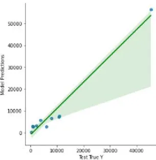
On the other hand, the linear GAM using the default value as parameter does not perform well, as from the prediction result, we found that the difference between the predictions and the actual output is very large, which is about 47% and 10% means the default value is not suitable to solve the problem well. From Figure 31, we can find that most of the prediction point is not close to the best fitting line, so it can show that the GAM with the default setting is not able to handle the data. GAM will also use the same elevation mode with Artificial Neural Network to measure performance.
Evaluation
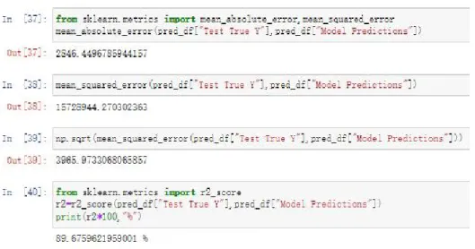
Since the aim of this project is to find the best performance between two models, we need to accurately implement both models so that these two models can work in the best state of both models. After using the best combination of parameters from GridSearchCV and we get a very interesting result. The average absolute error of the artificial neural network dropped from 2846.4497 to 2523.3070, which means that the prediction and the actual situation are more similar.
The R-square also increases about 3% and the prediction of the Artificial Neural Network will be more accurate. Figure 32 shows the MAE, RMSE and R-squared before ANN using the best combination of parameters, and Figure 34 shows the MAE, RMSE and R-squared after ANN using the best combination of parameters. The most dramatic change after model goodness-of-fit is Linear GAM, which Mean Absolute Error, Root Mean Square Error, and R-squared change significantly after using the best combination of parameters in Linear GAM.
The root mean square error is changed to 2043.4267 which means that the prediction distance and the line of best fit are closer to each other than the Artificial Neural Network. The R-squared of Linear GAM is also higher than Artificial Neural Network which 97.2592% can predict the most accurate prediction. Figure 33 shows the MAE, RMSE, and R-squared before GAM using the best combination of parameters, and Figure 33 shows the MAE, RMSE, and R-squared after GAM using the best combination of parameters.
Comment, Highlight, Model Selection
The three of the evaluation which are RMSE, MAE and R-squared also show that the Linear GAM performance is better than ANN as Linear has lower error and high R-squared. Besides that, GAM is not only the performance better than the ANN, but it has other advantages that can handle the non-linear and non-monotonic relationships between response and features. The ability to handle the non-linear complex data means that it does not need the polynomial to handle the complex data to fit the best fitting line to the complex data, so it can avoid the overfitting.
For example, before using the polynomial on one feature, the sample value is just 1000, but after using on the feature, the feature can become and it will cause the feature scale to become important to make that data in a comparable value range. Since it can handle the large data that can cause the non-linear result without using the polynomial, then the other developer or user who wants to use the model of this project, then it just needs to find a data set that has the same characteristic than we use on the GAM. This model can help the government of Malaysia to reduce the cases of the dengue as the accuracy of GAM is very high, so the government can provide the strategic effectively without using too much resources on meaningless strategic.
Conclusion
Prendinger, “Dengue Outbreak Forecasting Based on Disease Surveillance, Meteorological, and Socioeconomic Data,” BMC Infect. Uniqtech, “Multilayer perceptron (MLP) vs convolutional neural network in Deep Learning,” Data Science Bootcamp, Dec. 22, 2018. Available: https://medium.com/data-science-bootcamp/multilayer-perceptron-mlp-vs-convolutional -neural-network-in-deep-learning-c890f487a8f1.
Available: https://www.researchgate.net/publication/304069865_RELATIONSHIP_BE TWEEN_URBANIZATION_AND_DENGUE_HEMORRHAGIC_FEVER_INCIDEN CE_IN_SEMARANG_CITY. Using multiple data sources to estimate the economic costs of dengue in Malaysia,” Am. Adams, “How Artificial Intelligence Works - Becoming Human: The Journal of Artificial Intelligence,” Becoming Human: The Journal of Artificial Intelligence, 31 Oct. 2019.
Yasin, “Prediction of dengue incidence in northeast Malaysia from weather data using a general additive model,” Biomed Res. Salim et al., “Prediction of a dengue fever outbreak in Selangor, Malaysia using machine learning techniques,” Sci. Kamaludin, “Using artificial intelligence as a tool for dengue surveillance and prediction,” Journal of Applied Bioinformatics & Computational Biology , vol.
5, 2022. [Online] Available: https://www.scitechnol.com/peer-review/utilizing-artificial-intelligence-as-a-dengue-surveillance-and-prediction-tool-. Available at: