저작자표시-비영리-변경금지 2.0 대한민국 이용자는 아래의 조건을 따르는 경우에 한하여 자유롭게
l 이 저작물을 복제, 배포, 전송, 전시, 공연 및 방송할 수 있습니다. 다음과 같은 조건을 따라야 합니다:
l 귀하는, 이 저작물의 재이용이나 배포의 경우, 이 저작물에 적용된 이용허락조건 을 명확하게 나타내어야 합니다.
l 저작권자로부터 별도의 허가를 받으면 이러한 조건들은 적용되지 않습니다.
저작권법에 따른 이용자의 권리는 위의 내용에 의하여 영향을 받지 않습니다. 이것은 이용허락규약(Legal Code)을 이해하기 쉽게 요약한 것입니다.
Disclaimer
저작자표시. 귀하는 원저작자를 표시하여야 합니다.
비영리. 귀하는 이 저작물을 영리 목적으로 이용할 수 없습니다.
변경금지. 귀하는 이 저작물을 개작, 변형 또는 가공할 수 없습니다.
공학석사 학위논문
고분자전해질형 연료전지의 산소전달저항에 대한 모델링
Modeling of Oxygen Transport Resistance in PEM Fuel Cell
2 0 1 6 년 8 월
서울대학교 대학원 기계항공공항부 기계전공
이 유 일
Abstract
Modeling of Oxygen Transport Resistance in PEM Fuel Cell
Yoo-Il Lee Department of Mechanical and Aerospace Engineering The Graduate School Seoul National University
A Polymer Electrolyte Membrane (PEM) fuel cell is recognized as one of the promising clean energy sources that can replace internal combustion engine in the upcoming future. Unfortunately, the widespread usage of the fuel cell has not yet reached due to its high cost. Numerous studies have attempted to lower the overall cost of the fuel cell stack by analyzing and improving an individual cell. The studies can be roughly classified into two main streams of research.
1. Improvement in electrical conductivity by reducing the ionic resistance 2. Reduction of oxygen transport resistance
Recently, the latter has received significant attention. Unfortunately, the oxygen transport resistance is a tough parameter to obtain due to the difficulty involved in the measurement of oxygen concentration or a transfer rate. Therefore, the
modeling approach has attracted the scholars’ attention.
The aim of this study is to modify an existing quasi-three-dimensional model to analyze the oxygen transport resistance of the PEM fuel cell under various operating conditions. The model considered three difference kinds of transport mechanism: (1) molecular diffusion; (2) Knudsen diffusion; and (3) liquid-phase diffusion through ionomer film. Also, the model adopted a spherical agglomerate catalyst layer structure in order to estimate the oxygen transport phenomenon, more accurately.
The model was validated against two sets of gas diffusion layers (GDLs) by initially comparing the molecular diffusion resistance at the under-saturated condition and secondly, by comparing polarization curves at the fully saturated condition. The developed model was used to discern the effect of GDL structure on the oxygen transport resistance in a range of current density.
In conclusion, the modified model was able to separate and analyze the individual oxygen transport resistance in PEM fuel cell. The model shows the potential of evaluating the component of the cell by providing the results in quantitative values.
Keywords: PEM fuel cell, Oxygen transport resistance, Gas diffusion layer, Quasi-three-dimensional model
Student Number: 2014-21886
Table of Contents
Abstract ... i
List of Figures ... v
List of Tables ... vii
Nomenclatures ... viii
Chapter 1. Introduction ... 1
1.1. Background ... 1
1.2. Polymer Electrolyte Membrane (PEM) fuel cell... 3
1.3. Oxygen transport in PEM fuel cell ... 5
1.4. Oxygen transport resistance ... 8
1.5. Objective ... 9
Chapter 2. PEM fuel cell model description ... 10
2.1. Overview ... 10
2.2. Assumptions ... 11
2.3. Discretization ... 11
2.4. Conservation equations ... 14
2.5. Gas-phase mass transfer ... 14
2.6. Liquid-phase mass transfer... 18
2.7. Agglomerate model ... 20
2.8. Electrochemical model ... 22
2.9. Pressure drop ... 24
Chapter 3. PEM fuel cell model validation ... 26
3.1. Overview ... 26
3.2. GDL sample descriptions ... 26
3.3. Model parameters ... 30
3.4. Experimental setup ... 32
3.5. Limiting current density ... 35
3.5.1. Experimental conditions ... 35
3.5.2. Theory ... 36
3.5.3. Limiting current density ... 37
3.6. Polarization curves ... 40
Chapter 4. Results and Discussion ... 42
4.1. Under-saturated condition ... 42
4.1.1. Limiting current density ... 43
4.1.1.1. GDL A ... 43
4.1.1.2. GDL B ... 44
4.1.1.3. Comparison between A and B ... 45
4.2. Over-saturated condition ... 48
4.2.1. 1 A/cm
2vs. 2 A/cm
2... 48
4.2.1.1. GDL A ... 49
4.2.1.2. GDL B ... 50
4.2.1.3. Comparison ... 52
4.2.2. Oxygen transport resistance trends ... 55
4.2.2.1. GDL A ... 55
4.2.2.2. GDL B ... 57
4.2.2.3. Comparison between A and B ... 58
4.3. Further discussion ... 64
Chapter 5. Conclusion ... 66
Chapter 6. Bibliography ... 68
List of Figures
Figure 1. Schematic diagram of a PEM fuel cell adapted from O’Hayre et
al.[12] ... 4
Figure 2. Schematic description of oxygen transports in a cathode ... 5
Figure 3. Discretization of a PEM fuel cell model ... 13
Figure 4. Schematic diagram of anode/cathode control volumes ... 13
Figure 5. Schematic of an agglomerate model ... 20
Figure 6. A cross-sectional SEM image of GDL A ... 28
Figure 7. A cross-sectional SEM image of GDL B [48] ... 28
Figure 8. Pore size distributions of GDL A and GDL B ... 29
Figure 9. A schematic of the fuel cell station ... 33
Figure 10. A single PEM unit cell used in model validation experiments 33 Figure 11.The reduction of effective area using gaskets ... 34
Figure 12. Comparison of molecular diffusion resistance and other resistances between simulation and experiment (GDL A) ... 38
Figure 13. Comparison of molecular diffusion resistance and other resistances between simulation and experiment (GDL B) ... 39
Figure 14. Comparison of experimental polarization curve and simulated polarization curve (GDL A) ... 41
Figure 15. Comparison of experimental polarization curve and simulated polarization curve (GDL B) ... 41
Figure 16. Oxygen transport resistance of each component at under-saturated condition (GDL A) ... 44
Figure 17. Oxygen transport resistance of each component at under-saturated condition (GDL B) ... 45
Figure 18. Contribution of individual oxygen transport resistance at under- saturated condition (GDL A) ... 47
Figure 19. Contribution of individual oxygen transport resistance at under- saturated condition (GDL B) ... 47
Figure 20. Total oxygen transport resistance at 1 A/cm
2and 2 A/cm
2(GDL A)
... 49
Figure 21. Individual transport resistance at 1 A/cm
2and 2 A/cm
2(GDL A) ... 50 Figure 22. Total oxygen transport resistance at 1 A/cm
2and 2 A/cm2 (GDL
B) ... 51 Figure 23. Individual transport resistance at 1 A/cm
2and 2 A/cm
2(GDL A)
... 51
Figure 24. Contribution of individual resistance at 1A/cm2 and 2 A/cm2 for a) GDL A, b) GDL B ... 53
Figure 25. Water saturation profile at 1 A/cm
2and 2 A/cm
2for a) GDL A b) GDL B ... 54 Figure 26. Total oxygen transport resistance of GDL A ... 56 Figure 27. The change in individual oxygen transport resistance between 0.4
A/cm
2to 2.0 A/cm
2(GDL A) ... 56 Figure 28. Total oxygen transport resistance of GDL B ... 57 Figure 29. The change in individual oxygen transport resistance between 0.4
A/cm
2to 2.0 A/cm
2(GDL B) ... 58 Figure 30. Total oxygen transport resistance under various operating current
densities. ... 60 Figure 31. The change in ionomer resistance under various current densities
... 60 Figure 32. The change in water film resistance and water film thickness under
various current densities ... 61 Figure 33. The change in catalyst layer resistance under various current
densities ... 61 Figure 34. The change in MPL resistance under various current densities62 Figure 35. The change in substrate resistance under various current densities
... 62 Figure 36. The change in channel resistance under current densities ... 63 Figure 37. Comparison of activation overvoltage and Ohmic overvoltage
obtained from simulation ... 63
List of Tables
Table 1. Diffusion volume of simple molecules [31] ... 15
Table 2. Laminar friction constants for rectangular channel [47] ... 25
Table 3. Estimated physical parameters of GDL and catalyst layer ... 31
Table 4. Model parameters ... 32
Table 5. Dimension of channels ... 32
Table 6. Experimental condition for limiting current density tests ... 35
Table 7. Limiting current density results ... 38
Table 8. Experimental condition for polarization curves ... 40
Nomenclatures C concentration D diffusion coefficient DCF carbon fiber diameter Dh hydraulic diameter dp pore diameter F Faraday constant f friction coefficient g gravitational force H Henry’s Law constant hm mass transfer coefficient K permeability
KB Boltzmann constant Kn Knudsen number M molar mass
n number of electrons transferred Nagg agglomerate density, 1/m3 R gas constant
Re Reynolds number
Ro estimated solvent radius s water saturation
Sh Sherwood number x mole fraction Greek letters
α transfer coefficient δ thickness
ε porosity η overpotential κ conductivity λ mean free path μ viscosity
ν diffusion volume of molecules
Subscripts and superscripts act activation
agg agglomerate cl catalyst layer eff effective
g gas
ion ionomer knd Knudsen mix mixture ohm ohmic ref reference
w water
Abbreviations
PEM Polymer Electrolyte Membrane / Proton Exchange Membrane GDL Gas Diffusion Layer
PEN Penetration
MPL Microporous Layer CL Catalyst Layer
MEA Membrane Electrode Assembly RH Relative Humidity
OCV Open Circuit Voltage
SEM Scanning Electron Microscope MFC Mass Flow Controller
LPM Liter Per Minute SR Stoichiometric Ratio
ICE Internal Combustion Engine
Chapter 1. Introduction
1.1. Background
During the late 18th and early 19th centuries in Britain, there was a milestone in human history, the Industrial Revolution. The utilization of fossil fuel and the transition from hand production methods to machine manufacture have modernized our way of living beyond imaginations. However, the indiscreet use of fossil fuel and the lack of knowledge on incidental effects on the environment have dramatically polluted the earth’s atmosphere and resulted in “global warming”.
Fortunately, for the last few decades, a large number of countries have considered the climate change caused by global warming as a single biggest environmental and humanitarian issue of our time. Since transportation is regarded as one of the main sources of air pollution (including greenhouse gas emission), legislations and regulations on automotive vehicle emissions have been established and continuously enhancing to restrain and minimize the environmental damage [1]. Accordingly, automotive manufacturers have been developing and improving the combustion engine technologies to satisfy the current fuel and emission standards and other enhanced standards to come. However, as relevant regulations become increasingly stringent, it seems difficult to meet the fuel and emission standards solely with a conventional combustion engine. This prediction has been supported by the series of emission-cheating and fuel mileage scandal from major automakers [2, 3]. As a result, alternative ways of powering vehicles have devised in both entrepreneur’s and customer’s minds.
One of the promising replacement for internal combustion engine (ICE) is a fuel cell.
Unlike an ICE, which produces harmful exhaust gas, a polymer electrolyte membrane (PEM) fuel cell operates at a low temperature (~80℃) and produce water and heat only. Moreover, provided that the hydrogen is produced using renewable energy, it is a self-sustainable energy source without any damage to the environment.
Besides the eco-friendly aspect, fuel cells have a few advantages over ICEs. Firstly, fuel cells directly generate electricity through an electrochemical reaction; hence they do not require any moving components and offers opportunities to make the system more reliable and quiet. Additionally, they avoid Carnot limitation and achieves much higher efficiency. However, the commercialization of fuel-cell powered vehicles has been delayed due to its durability and expensiveness concerns [4].
Consequently, the comprehensive researches have been carried out to improve the overall output of a cell while ensuring both mechanical and chemical durability of an individual fuel cell component, for instance, a gas diffusion layer (GDL), a microporous layer (MPL) and so on [5-9]. Furthermore, substantial efforts have been made to lower the price of the stack to the ICE level by developing non-precious metal catalysts to replace the expensive platinum catalysts [10, 11]. As the result of these continuous studies, a significant improvement on PEM fuel cells have been made, and the commercialization of fuel cells now is one step closer.
1.2. Polymer Electrolyte Membrane (PEM) fuel cell
A PEM fuel cell is a type of fuel cell that utilizes a polymer membrane as an electrolyte. The main advantage of this kind of fuel cell is the ability to operate at a relatively low temperature (~80˚C) with high power density. Therefore, a PEM fuel cell has been recognized as a choice for an alternative portable power source including the automotive application.
The fundamental principle of fuel cells is straightforward. It is the reverse reaction of water electrolysis as listed on the following equation.
𝐻2+1
2𝑂2→ 𝐻2𝑂 (1.1)
To harness the electrical energy from this reaction, polymer electrolyte membranes are used. The noticeable feature of these membranes is the ability to allow the movement of protons while blocking electrons. The division of protons and electrons paths allows an external load circuit to be created. As shown in Figure 1, hydrogen oxidation occurs at the anode, and hydrogen ions and electrons travel through their individual path to react with oxygen at the cathode. Hence, the movement of the electron grants the utilization of electrical energy generated from the electrochemical reaction.
Figure 1. Schematic diagram of a PEM fuel cell adapted from O’Hayre et al.[12]
The voltage output of the cell is sensitively affected by the catalyst condition.
According to the Nernst equation and Butler-Volmer equation, the concentration of reactant gas at the catalyst surface severely influences the cell performance; hence, to achieve high reactant concentration, the cell should possess the ability to transport the reactant gas effectively, as well as to efficiently remove any excessive liquid water. The most of the focus on the reactant transport is limited to the cathode due to the following reasons. Firstly, the water is produced at the cathode catalyst.
Secondly, the reactant fuel for the cathode is usually the air that only consists of 21%
of oxygen. Lastly, the rate of oxygen reduction reaction is much slower than that of the hydrogen oxidation reaction. Therefore, numerous studies have been conducted to improve the cell performance by focusing on oxygen transport phenomenon.
e- e-
H+ H+
1.3. Oxygen transport in PEM fuel cell
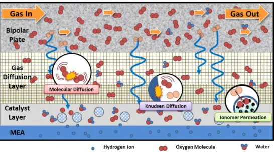
The oxygen transport from the cathode flow-field to the platinum surface in the catalyst layer is conceptualized as shown in Figure 2. The transport of the oxygen molecules can be divided into the following components:
1) Flow-field region.
2) GDL with MPL region.
3) Catalyst layer region.
Figure 2. Schematic description of oxygen transports in a cathode
Due to the difference in physical properties, the primary oxygen transport mechanism for each layer might vary. At the flow-fields, a reactant gas is subjected to convective force and transported along the channel at a rapid rate. As the gas enters the substrate in GDL, the mode of transport changes from convection to diffusion.
The average pore diameter of the substrate is much larger than the mean free path of
gas molecules. Consequently, the interaction between gas molecules becomes the main driving force of diffusion, that is, molecular diffusion. As oxygen passes through the substrate of GDL, it encounters much smaller pores at the MPL of GDL and the catalyst layer. As the pore diameter approximates to the figure of mean free path of the gas molecules, the molecules start to collide frequently with the diffusion medium. The diffusion process, caused by the collision of molecules and the medium, is called Knudsen diffusion. As a result, the diffusion at the MPL and the catalyst layer is no longer solely molecular diffusion, but the combination of molecular and Knudsen diffusion. After reaching the catalyst agglomerate, oxygen has to be dissolved to permeate the ionomer covering the agglomerate. These are the oxygen transport mechanisms and a brief idea of oxygen transport resistance for each component.
In recent years, numerous researches on fuel cell components such as GDLs, catalysts, and bipolar plates, have been conducted to reduce the oxygen transport resistance and increase the operating power range of the cell [13-18]. One of the attempts to minimize the oxygen transport resistance focuses on the flow-field. A conventional flow-field is a graphite plate carved in channels. The reduction of the rib area decreases the transport resistance at the channel-GDL interface and attributes to a higher distribution of reactant gas. Therefore, it was reported that minimizing the widths of the channels and the ribs increases a cell performance [19].
Kumar and Reddy [18] had replaced the channel-inscribed flow-field with metal foam to remove the existence of ribs. Similar research regarding the porous flow distributor was attempted [20]. Despite the positive effect on the interfacial area
Firstly, the introduction of the foam structure significantly increases the pressure drop, in other words, it requires a higher power compressor that increases the axillary power consumption. Secondly, even with the higher compressor, a substantial amount of residual water tends to stay in pores, reducing both stack performance and stability. By combining the benefits of the conventional flow-field and porous flow- field, a three-dimensional fine-mesh flow-field was developed by Toyota Motors [21]. The developed flow-field separated the airway and waterway for the purpose of promoting oxygen diffusion at the catalyst layer and expelling the generated water to the outer surface of the 3D fine mesh flow.
Meanwhile, some have employed a variation in GDL property in the through-plane direction to endorse the removal of excess liquid water at high humidity conditions, and at the same time, maintain higher membrane water contents at low humidity conditions [13]. Others have removed GDLs to improve the cell performance as the porous field could compensate their absence [22].
1.4. Oxygen transport resistance
The reduction in oxygen transport resistances is the key to a higher cell performance.
Hence, there have been studies concerned specifically with the measurement of oxygen transport resistance in each component. Beuscher [23] suggested a simple mean of measuring mass transport resistance using limiting current densities. By changing carrier gases and the number of GDLs, the author found that the GDL was responsible for about 25% of the total transport resistance. In addition, the analysis reveals that the resistance from Knudsen diffusion, ionomer permeation, and water film accounted 56% of the total resistance. Baker et al. [24] also separated the oxygen transport resistance into the channel, substrate, MPL and other resistance. The authors conducted the experiments at the condition when the cell was adequately humidified, but no liquid water condensed. In this study, the contributions of the diffusion medium, channel, microporous layer, and others were 53%, 24%, 8% and 15%, respectively. In 2011, Nonoyama et al. [25] divided the total oxygen transport resistance into the molecular, Knudsen and ionomer film resistance by varying operating temperature and balance gas. The authors concluded that the ionomer resistance took significant portions of transport resistance at low temperature and humidity conditions.
An experimental approach to the measurement of oxygen transport resistance of individual layer requires a series of experiments. In addition, due to the difficulty associated with the liquid water effect, the majority of the published experiments were limited to under-saturated conditions. Therefore, to overcome these obstacles, a computer modeling approach is recommended as one of the solutions.
1.5. Objective
The main purpose of the study is to modify an existing quasi-three-dimensional model to estimate the oxygen transport resistance by each component under various operating conditions.
To properly predict the oxygen transport resistance, substantial revisions were made on the model created and modified by Kang [26] and Park [27]. Originally, the PEM fuel cell model was developed as a part of the integrated PEM fuel cell electrical vehicle system. As a result, the transport phenomena was simplified using binary diffusion coefficients and thin catalyst layer models. To adequately capture the real transport phenomenon, the model had undergone major revisions on the oxygen transport mechanism to consider multicomponent mixture, Knudsen diffusion, and agglomerate catalyst model. The developed model was firstly validated against the experimental results by comparing the limiting current density results of two-percent oxygen with nitrogen and one with helium diluent. This validation confirmed the ability of the developed model to estimate the total oxygen transport resistance and the contribution of molecular diffusion resistance from the total. Secondly, the current-voltage curves results were juxtaposed to verify its capability to imitate the transport phenomena on normal operating conditions.
In this study, the current density was varied to examine the effect of the operating point on the transport resistance. Moreover, two different sets of GDLs with distinct physical properties namely, GDL A and GDL B were analyzed to observe the effect of the GDL on the individual oxygen transport resistance.
Chapter 2. PEM fuel cell model description
2.1. Overview
The model used in this study was a quasi-three-dimensional dynamic model based on MATLAB®/Simulink® platform. A one-dimensional PEM fuel cell node was created in through-plane direction, then it was reproduced to be arranged in an in- plane direction to form a quasi-three-dimensional model. This approach allowed the model to modestly reflect the spatial characteristics of the cell along the channel with lesser computation power, compared to the full-scale three-dimensional model [27].
Several changes to the previous model were made to accurately compute the oxygen transport resistance during various cell operation conditions. The introduction to the previous model are as follows:
1) Multicomponent diffusion 2) Knudsen diffusion, and
3) Agglomerate catalyst layer model
In addition, the control of inlet oxygen concentration and the selection of the inert gas were supplemented to provide the mean of comparing acquired simulation results against empirical results.
2.2. Assumptions
A number of assumptions were employed to decrease the computational time without significantly degrading the accuracy of the result. In addition to the major assumptions adopted by Kang [26], the following assumptions were made to reflect the agglomerate structure.
1. Liquid water in the catalyst covers the agglomerates and create a water coating layer [28].
2. The agglomerates are located near catalyst-MEA interface.
3. The transport inside the agglomerates is ignored.
2.3. Discretization
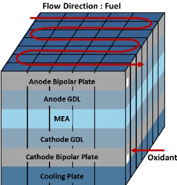
A PEM fuel cell model was discretized to into several control volumes to sufficiently describe the behavior of a cell. Firstly, the fuel cell was discretized in a direction perpendicular to the gas stream, and then in the flow direction to capture and imitate the mass transport phenomena such as convection, diffusion, and capillary water flux (Figure 3). A PEM fuel cell is consisted of bipolar plates with channels, GDLs with MPL, and a membrane-electrode-assembly (MEA). The minimum of one control volume was allotted to apprehend the mass and heat transfer for each component. In the previous studies, the temperature of the cell was manipulated by the coolant flowing through the flow channels. However, in this study, the temperature of the cell was regulated by heating poles, plunged into the holes in bipolar plates. Hence, the needs for coolant channels and coolant plates were unnecessary. Therefore, those were suppressed to reduce the computation time. MPLs are in contact with MEA and
have a pore size around hundred nanometers while substrates have near hundred micrometers. Accordingly, the mass transport phenomenon such as oxygen diffusion and capillary flux is highly affected by its location on GDL. As a result, the control volumes of eight were selected for each GDL to replicate the variation of the physical properties as shown in Figure 4. Noticeable, five control volumes were assigned to the substrate while the MPL were assigned with three. The discretization along the flow direction influences the cell performance by reflecting the change in gas compositions due to fuel depletion and water generation. It was intimated that the detail discretization of the cell would increase the accuracy of the model. However, it would significantly put a strain on the PEM model and demand a higher computing power. Since the model was originally developed for the control and system design tools [29], the maximum discretization number of 35 was limited to ensure the fast calculation speed and the model compactness.
Figure 3. Discretization of a PEM fuel cell model
Figure 4. Schematic diagram of anode/cathode control volumes
2.4. Conservation equations
For each control volume, conservation of energy and conservation of species were employed to determine the local temperatures, mole fractions, and their flux.
Specifically, Newton’s law of cooling and Fourier’s law were used to obtain the heat rate. The “perfect mixing” assumptions were made for all control volume in the calculation of molar flux. More detailed descriptions of conservation equations can be found in Reference [26].
2.5. Gas-phase mass transfer
All the reactants of the PEM fuel cell were supplied in gaseous form. Consequently, the comprehensive modeling of gas-phase mass transfer was a critical factor in accurately estimating the oxygen transport resistance. The previous model utilized binary diffusion coefficient constants and used the saturation of control volume to modify the diffusion coefficients. Even though it was able to imitate the effects of saturation,
it could not reflect the change in diffusion coefficient due to the change in gas composition. In addition, preceding model ignored Knudsen diffusion and ionomer resistance. For these reasons, new equations were introduced to estimate the effective diffusion coefficient of each control volume using proper diffusion mechanism. In the following subsections, the method of selecting appropriate oxygen transport mechanism and calculating effective coefficient will be elaborated.
2.5.1 Diffusion Coefficient
The diffusion coefficient of gas is affected by a number of factors such as a temperature, pressure, composition and property of the diffusion medium. The molecular diffusion coefficient was calculated using both the binary diffusion equation and the multicomponent mixture gas equation for each control volume. For MPLs and catalyst layers, the effective diffusion coefficients were computed by harmonic averaging of molecular diffusion and Knudsen diffusion.
Firstly, the binary gas diffusion coefficient was predicted using the equation developed by Fuller et al. [30].
𝐷𝐴𝐵(𝑐𝑚2/𝑠) =1.00×10
−3𝑇1.75( 1
𝑀𝐴+ 1
𝑀𝐵)
0.5
𝑃[(∑ 𝑣𝐴)13+(∑ 𝑣𝐵)13]
2 (2.1)
The unit for temperatures and pressures are in Kevin and atmosphere, respectively.
M is the molar mass of the molecule.
𝑣 is the diffusion volume of molecules.
Table 1. Diffusion volume of simple molecules [31]
Species Diffusion Volume Species Diffusion Volume
Nitrogen 17.9 Water 12.7
Helium 2.88 Hydrogen 7.07
Oxygen 16.6
Secondly, a multicomponent equation was used to acknowledge the effect of the gas composition. In a cathode side, nitrogen, oxygen, and water vapor gas exist, making a tertiary gas composition. Thus, the molecular diffusion coefficient in mixture gas was estimated by the relation verified by Fairbanks and Wilke [32].
𝐷𝐴−𝑚𝑖𝑥 = 𝑦𝐵 1−𝑦𝐴
𝐷𝐴𝐵+𝑦𝐶
𝐷𝐴𝐶+𝑦𝐷
𝐷𝐴𝐷+⋯ (2.2)
Thirdly, Knudsen number was used as a criterion to determine the appropriate diffusion mechanism for each control volume.
𝑘𝑛= 𝜆
𝑑𝑝 {
𝑘𝑛< 0.01 Molecular region 0.01 ≤ 𝑘𝑛≤ 10 Transition region
𝑘𝑛> 10 Knudsen region
(2.3)
In the calculation of Knudsen number, mean free path in mixture gas was used [33].
𝜆𝑖 = 1
∑ 𝜋(𝑟𝑖+𝑟𝑗)2𝑛𝑗√1+(𝑚𝑖
𝑚𝑗)
𝑁𝑗=1
(2.4)
Then, to calculate the diffusion coefficient for transition or Knudsen region, the following equation was used to derive the Knudsen diffusion coefficient [34].
𝐷𝑖−𝑘𝑛𝑢𝑑=𝑑𝑝
3 √8𝑅𝑇𝜋𝑀
𝑖 (2.5)
During the transition region, both diffusion mechanism should be considered. Thus, Bosanquet formula was used to include both contribution as below [35].
𝐷𝑐𝑜𝑚𝑏𝑖𝑛𝑒𝑑= ( 1
𝐷𝑖−𝑚𝑖𝑥+ 1
𝐷𝑖−𝑘𝑛𝑢𝑑)−1(𝑓𝑜𝑟 0.01 ≤ 𝐾𝑛≤ 10) (2.6)
2.5.2 Gas-phase mass transfer in GDL
For convective mass transfer between the gas channel and GDL, the following equations were used [36].
𝛷⃗⃗ 𝑐𝑜𝑛𝑣 = ℎ⃗ 𝑚𝐴(𝐶𝑖,𝑐ℎ𝑎𝑛𝑛𝑒𝑙− 𝐶𝑖,𝐺𝐷𝐿) (2.7) ℎ⃗ 𝑚=𝑆ℎ∙𝐷⃗⃗ 𝑚
𝐷ℎ (2.8)
For diffusion mass transfer, the diffusion length of the porous material is affected by the tortuosity of the material. The estimation of the tortuosity is challenging due to the randomness of the carbon fiber stacks; hence, Bruggeman correlation was used to estimate the effect of the tortuosity [37].
𝐷⃗⃗ 𝑚𝑒𝑓𝑓= [𝜀(1 − 𝑠)]1.5𝐷⃗⃗ 𝑚𝑔 (2.9)
Diffusion mass transfer rate was modeled based on Darcy’s equation as the following equation.
𝛷⃗⃗ 𝑑𝑖𝑓𝑓 =𝐷⃗⃗ 𝑚
𝑒𝑓𝑓𝐴
𝑡 (𝐶𝑖+1− 𝐶𝑖) (2.10)
2.6. Liquid-phase mass transfer
The management of the liquid water in PEM fuel cells are vital in achieving high performance. The formation of liquid water blocks the pores in the catalyst layer and covers the agglomerate with water films. Consequently, the oxygen transfer rate decreases and cell voltage deteriorates. On the contrary, the presence of liquid water at membrane causes a sharp change in water uptake, as known as Schroeder’s paradox, and helps to lower the membrane conductivity [37]. Therefore, the control of liquid water is essential in determining accurate cell voltage; hence the liquid water transfer was prudently modeled using the multiphase mixture formation, developed by Wang et al. [38].
In this model, most of the equation relating to the liquid-phase mass transfer is the same as previous Kang’s model [26]. However, few modifications were made to improve the prediction of the liquid water flux.
Firstly, the relative permeability model was changed as it was reported that the following relation is more appropriate for diffusion medium [39].
𝑘𝑟𝑙= 𝑠2.16, 𝑘𝑟𝑔 = (1 − 𝑠)2.16 (2.11)
Secondly, the method of estimating the permeability was replaced. The permeability is often calculated using the Kozeny-Carman relation [40] using pore diameter and porosity. However, it is not suitable for fibrous materials such as GDLs, and it cannot accurately calculate the permeability in the transition flow regimes. Therefore, the
permeability of the fibrous porous media was calculated using the equation formulated by Jeong et al. [41].
𝐾
𝐷𝐶𝐹2 = exp {𝐶1ln ( 𝜀
11 3
(1−𝜀)2) − 𝐶2} (2.12) {𝐶1= 0.7128 − 0.4953𝐾𝑛
𝐶2= 1.974 − 4.2892
Thirdly, the water diffusion coefficient was halved. The equation used to calculate the water diffusion coefficient in the membrane was for Nafion™ membrane.
However, the membranes from Gore company were used in this study. Therefore, the previous equation was not directly applicable. In 2007, Ye and Yang [42]
experimentally measured the water diffusion coefficient of Gore-Select membrane and found that it was roughly the half of Nafion membrane. Therefore, in this study, the membrane was assumed to be consisted of 50% of Nafion materials.
𝐷𝑤,𝑒𝑓𝑓 = 0.5𝐷𝑤 (2.13)
2.7. Agglomerate model
The preceding model assumed that the catalyst layer is thin, and the structure of its layer could be ignored. However, experimental results revealed that the oxygen transport resistance in a catalyst layer contributes to the 15% of the total dry transport resistance [24]. Therefore, the porous electrode model was introduced to reflect the agglomerate structure in oxygen transport phenomena while assuming uniform concentration and potential across the layer [36]. As shown in Figure 5, it is modeled that the ionomer film entirely covers the agglomerate surface. Additionally, any residing liquid water in the catalyst layer was assumed to form water films around ionomers as shown in the equation below [28].
δw = √(𝑟𝑎𝑔𝑔+ 𝛿𝑖𝑜𝑛)3+ 3𝑠𝜀𝑐𝑙
4𝜋𝑁𝑎𝑔𝑔
3 − (𝑟𝑎𝑔𝑔+ 𝛿𝑖𝑜𝑛) (2.14)
To reach the reaction site, oxygen molecules have to be dissolved and transported through one or two layers. Since the oxygen molecules are transported across a phase boundary, the discontinuous molar concentration occurs at the phase interface. The concentration discontinuity was modeled with Henry’s constants obtained by experimental results [28]:
𝐻𝑂2(𝑃𝑎. 𝑚3. 𝑚𝑜𝑙−1) = 0.11552 𝑒𝑥𝑝 (14.1 + 0.0302𝜆 −666
𝑇 ) (2.15)
The liquid-phase diffusion of oxygen molecules was estimated using the Stokes- Einstein equation:
𝐷𝑂2−𝐻2𝑂 =6𝜋𝜇𝑅𝑘𝐵𝑇
𝑜 (2.16)
Ro is the estimated solvent radius, and the value for oxygen is 1.734 ångström.
The oxygen diffusivity in Nafion® ionomer was corrected by Marr and Li [43] as
𝐷𝑂2−𝑀𝑒𝑓𝑓 = 1.3926 × 10⁻¹⁰𝜆0.708𝑒𝑥𝑝 (𝑇 − 273.15 106.65 )
−1.6461 × 10⁻¹⁰𝜆0.708+ 5.2 × 10⁻¹⁰ (2.17)
2.8. Electrochemical model
The nodal voltage was calculated by subtracting the activation overvoltage and ohmic overvoltage from the open circuit voltage.
𝑉𝑐𝑒𝑙𝑙 = 𝑉𝑂𝐶𝑉− 𝜂𝑎𝑐𝑡− 𝜂𝑜ℎ𝑚 (2.18)
The previous model used the theoretical reversible voltage as a constant term of Nernst equation. However, the theoretical reversible voltage tends to over-predict the open circuit voltage, as it does not consider the effects of voltage drop due to the fuel crossover and the mixed potential of the Pt/PtO catalyst surface [44].
Therefore, the calculation of the open circuit voltage was correlated by Eq. (2.19) [45] and the Nernst equation.
𝑉𝑂𝐶+= 0.0025T + 0.2329 (2.19) 𝑉𝑂𝐶𝑉= Voc++∆𝑠̂
𝑛𝐹(𝑇 − 𝑇0) −𝑅𝑇
𝑛𝐹ln∏ 𝑎𝑝𝑟𝑜𝑑𝑢𝑐𝑡𝑠
𝑣𝑖
∏ 𝑎𝑟𝑒𝑎𝑐𝑡𝑎𝑛𝑡𝑠𝑣𝑖 (2.20)
For activation overvoltage, only the cathodic reaction kinetics was considered, and the simplified form of Butler-Volmer equation was used. Due to the introduction of the water film, the saturation effects were removed from the previous model to avoid redundancy.
𝜂𝑎𝑐𝑡=𝑅𝑇
𝛼𝐹ln (𝑗
𝑗𝑜 𝐶𝑂2
𝑟𝑒𝑓
𝐶𝑂2) (2.21)
The ionic conductivity of Nafion is dependent on water content as shown in Eq. (2.22) [12]. The proton conductivity of the membrane was assumed to be the half of the Nafion membrane.
𝜅 = (0.005139𝜆 − 0.00326) exp (1268 ( 1
303−1
𝑇)) (2.22) 𝜅𝑒𝑓𝑓 = 0.5𝜅 (2.23)
Then, the sum of the resistance was expressed by the following equation.
𝑅𝑜ℎ𝑚=𝑡𝑚𝑒𝑎
𝜅𝑒𝑓𝑓+2𝑡𝐺𝐷𝐿
𝜎 + 𝑅𝑐𝑜𝑛𝑡𝑎𝑐𝑡 (2.24)
Using the Ohm’s law, the ohmic overvoltage was obtained.
𝜂𝑜ℎ𝑚= 𝐼𝑅𝑜ℎ𝑚 (2.25)
Due to the equipotential electrode assumption, entire nodes of the cell had to be the identical value. Thus, the nodal current was iterated until all the cell voltage was equal, satisfying the following equation.
𝑉𝑐𝑒𝑙𝑙 = 𝑉𝑛𝑜𝑑𝑒 = ∑ 𝐼𝑛𝑜𝑑𝑒𝑅 (2.26)
2.9. Pressure drop
The gas pressure in the PEM fuel cell varies node by node due to the following reasons. Firstly, the electrochemical reaction alters the number of the molecules in each channel. Secondly, the supplied gas experiences a frictional force as it travels through the flow channel. The former is negligible and not reflected in the model.
However, pressure drop due to the frictional shear force could not be overlooked.
Therefore, the calculation of Reynolds number and the friction coefficient were calculated using Eq. (2.27) to Eq. (2.28). For friction coefficients for the turbulent flow, Filonenko equation was used, presuming the smooth surface [46].
1. Laminar Flow:
𝑅𝑒 = 𝜌𝜈𝐷𝐻
𝜇 (2.27)
𝑅𝑒 < 2300, 𝑓 =𝑓𝑅𝑒
𝑅𝑒 (2.28)
2. Turbulent Flow
𝑅𝑒 ≥ 2300, 𝐷𝑒𝑓𝑓= [64
𝑓𝑅𝑒] 𝐷𝐻 (2.29)
𝑅𝑒𝑒𝑓𝑓=𝜌𝜈𝐷𝑒𝑓𝑓
𝜇 (2.30)
𝑓 = (1.82 log10𝑅𝑒 − 1.64)−2 (2.31)
Table 2. Laminar friction constants for rectangular channel [47]
height / width fRe height / width fRe
0.0 96.00 0.25 72.93
0.05 89.91 0.4 65.47
0.1 84.68 0.5 62.19
0.125 82.34 0.75 57.89
0.167 78.81 1.0 56.91
In addition to the major head loss, minor head losses were introduced in this model to capture the effect of the pressure drop around the sharp corners. Through Eq. (2.32) to Eq. (2.35), the major and minor head losses were calculated, and the pressure drop for each node was computed.
hf= 𝑓 𝐿
𝐷ℎ 𝑣2
2𝑔 (2.32)
h𝑚= 𝑣2
2𝑔Σ𝐾 (2.33)
h𝑡𝑜𝑡𝑎𝑙 = ℎ𝑓+ ℎ𝑚 (2.34)
Δ𝑝 = 𝜌𝑔ℎ𝑡𝑜𝑡𝑎𝑙 (2.35)
Chapter 3. PEM fuel cell model validation
3.1. Overview
Model validation was conducted by comparing the limiting current result and current-voltage curve. Firstly, the limiting current density of the cells was obtained both empirically and theoretically by using two-percent oxygen with nitrogen and helium diluent. The comparison of limiting current density results verified the model’s ability to analyze the molecular diffusion resistance from other resistance at under-saturated water vapor condition. Secondly, the model was simulated to draw a polarization curve at fully humidified condition. The polarization curves of both simulation and experimental results were compared to confirm the proper estimation of oxygen transport resistance at over-saturated condition.
3.2. GDL sample descriptions
In this study, two sets of GDLs with distinct physical properties were selected to observe the oxygen transport resistance of the individual component. Both GDL samples were the carbon paper-type GDL with an MPL coating. They were manufactured by different companies and will be referred as “A” and “B”. Due to the number of the speculations made on the physical properties, the sample name, as well as the name of the company were undisclosed.
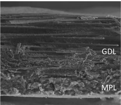
Scanning electron microscope (SEM) images clearly revealed a noticeable difference between those two GDLs (Figures 6 and 7). Carbon fibers in GDL A were straight and appeared rigid. By contrast, fibers in GDL looked more flexible. As suspected from the SEM image, GDL A was more brittle than GDL B, making it more vulnerable to the impact. In addition, GDL A seemed to have a larger void volume in substrate (Figure 6). Another noticeable difference was the appearances of the MPL. The images indicated that MPLs of both GDLs are undoubtedly dissimilar which may lead to the change in oxygen transport resistance. Moreover, GDL B showed a clear borderline between MPL and substrate. In opposition to this, MPL of the GDL A sample penetrated deeply into the substrate area, blurring the MPL and substrate borderline as observed in Figure 6.
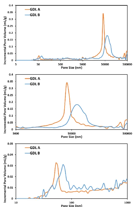
The pore size distributions of both GDLs were obtained using a mercury porosimetry.
Two distinct peaks were seen in the entire pore size range: one peak around 70 nanometers, and the other around 50 micrometers (Figure 8). The smaller pore size peaks were generated by MPL, and it can be characterized as the representative MPL pore size. In a similar fashion, the larger size peaks were produced by carbon fibers in substrates. The results indicated that the pore sizes of MPL and substrate for GDL A and GDL B were 56.3 nm, 70.1 nm, 40.5 μm and 60.5 μm, respectively. At the same time, porosimetry informed that the porosity of the GDL A was 5.71% higher than that of GDL B. It appeared that GDL A was specifically designed to possess the smaller pore size yet exhibit higher porosity.
Figure 6. A cross-sectional SEM image of GDL A
Figure 7. A cross-sectional SEM image of GDL B [48]
Figure 8. Pore size distributions of GDL A and GDL B
3.3. Model parameters
The model parameters were carefully chosen to mimic the behavior of the fuel cell operation. GDLs are subjected to compressive forces during the cell assembly process and the physical properties such as porosity, thickness and pore size distribution changes. Therefore, the properties such as porosity, thickness, and pore size were measured at pristine conditions and then the severity of the compression effect on each property was judged, and the model inputs were chosen cautiously.
The total GDL thickness was measured with micrometers, and the thickness of the MPL was estimated from the SEM image. The substrate part was assumed to be the only compressible materials due to the high porosity, and compressed substrate thickness was estimated. The measurement on the local porosity is challenging as MPL cannot stand alone. In 2010, Ostadi et al. [49] attained local MPL porosity of 40% using FIB/SEM nano-tomographic 3D reconstruction. In this study, the local porosities were reasonably speculated using the overall GDL porosity results from mercury porosimetry and the MPL porosity of 40%. The average pore size of MPL and substrates were chosen to be the peak values in the pore size distribution data without taking into account the decrease in pore size during the cell assembly. The internal contact angle of GDLs controls the capillary water flux. Therefore, the accurate value for contact angle is critical in simulating water saturation effect.
Due to the difficulty involve in the measurement of agglomerate properties, the values were estimated from the work of others. Firstly, the ionomer film was reported to have a thickness between 3 to 10 nm [50]. Therefore, the ionomer thickness was
selected to be the value of 7 nanometers as stated by Lopez-Haro et al. [51]. The typical agglomerate size is known to be in the range of 50-100 nm [52]. For the agglomerate radius, 87.5 nm was chosen, considering the selected ionomer film thickness.
The catalyst layer was estimated by measuring the total MEA thickness and subtracting ionomer thickness which was provided by the manufacturer. Two peaks were observed in the BET measurement, and they were believed to be responsible for the inter-agglomerate pore size and the intra-agglomerate pore size. However, the intra-agglomerate structure was not considered in this study; hence the average mean pore size of 48.7 nm was used.
Table 3. Estimated physical parameters of GDL and catalyst layer
Description GDL A GDL B
Thickness (μm)
Substrates 214 227
MPLs 30 45
Catalyst Layer 7
Porosity (%)
Substrates 85 74
MPLs 40
Catalyst Layer 36
Pore size (nm)
Substrates 40,500 60,500
MPLs 56.3 70.1
Catalyst Layer 48.7
Internal Contact Angle (degrees)
Substrates 122.5 118 [48]
MPLs 140.5 99 [48]
Table 4. Model parameters
Parameter Value Ref.
Transfer Coefficient 0.567 [53]
Exchange Current Density 4.956e-5 A/cm2 [43]
No of agglomerate 1.01e19 m-3 Est.
Agglomerate Radius 87.5 nm Est.
Ionomer film thickness 7 nm [51]
3.4. Experimental setup
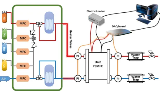
A fuel cell station used in this study is as shown in Figure 9. It was equipped with five individual mass flow controllers (MFCs) to manipulate the composition of inlet gas. For the humidification of the reactant gas, membrane humidifiers were used.
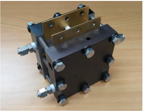
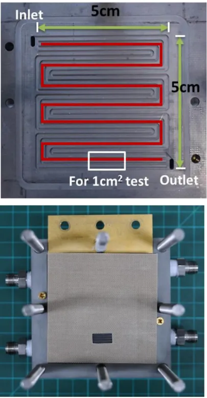
Cells were tested with Kikusui electronic load (PLZ664WA), and the corresponding voltage outputs were measured with National Instrument data acquisition board (USB6009) for faster sampling and more accurate measurement. The high-purity gases with over 99.995% purity were used in the experiments. For air, multiple filters and a pneumatic dryer were utilized to remove unwanted particles and moist before entering the station. 25cm2 unit cells with quadruple serpentine channels were used in the study. The dimensions of the channels are presented in Table 5. For the limiting current density tests, the effective area was decreased to 1cm2 by covering the rest of the effective area with the gasket as shown in Figure 11.
Table 5. Dimension of channels
Channel Width Channel Depth
Anode 1 mm 0.4 mm
Cathode 1 mm 0.5 mm
Figure 9. A schematic of the fuel cell station
Figure 10. A single PEM unit cell used in model validation experiments
Figure 11.The reduction of effective area using gaskets
3.5. Limiting current density
3.5.1. Experimental conditions
The purpose of the limiting current density test was to obtain the total oxygen transport resistance and isolate the contribution of molecular diffusion resistance from the obtained value. For valid results, the cell needed to be operated in the under- saturation condition. At the same time, a sufficient amount of water vapor was necessary to ensure the limiting current result from mass transport, not from ohmic overvoltage. To achieve this condition, the two-percent oxygen concentration was partially humidified to be used as the inlet gas. Additionally, the active area was reduced to 1cm2, and the flow rate was set to a high value to minimize the oxygen depletion effect. Two sets of GDLs with the same GORE™ PRIMEA® 5730 MEA were used in this experiments.
Table 6. Experimental condition for limiting current density tests
Parameter Condition
Test Mode Voltage Control (1.0V→0.05V, 90 mV/s) Active Area 1cm2 (1.4 cm by 0.715 cm)
No. Parallel channel 4
Temperature / Pressure 65 ℃ / 1atm.
Relative humidity 90 %
Oxygen Concentration 2 %
Diluent gas Nitrogen / Helium
Flow Rate 0.2 / 2.54 LPM (Anode/Cathode, SR>10)
GDL GDL A / GDL B
MEA GORE™ PRIMEA® 5730
3.5.2. Theory
The total oxygen transport resistance can be mathematically expressed as:
𝑅𝑂2𝑇𝑜𝑡𝑎𝑙= (𝐶𝑂2,𝑐ℎ− 𝐶𝑂2,𝑃𝑡) 𝑁⁄ 𝑂2 (3.1)
Unfortunately, the measurement of neither oxygen concentration at a platinum surface nor an oxygen transport rate is not readily available. However, at limiting current density, the oxygen concentration on the platinum surface becomes zero, and the oxygen transport rate matches the oxygen consumption rate. Then, by equating oxygen transport rate and oxygen reduction rate, total mass transport resistance can be obtained using Eq. (3.2).
(3.2)
Using modestly humidified low oxygen concentration gas with the small active area, it can avoid any liquid water droplet formation or water film over agglomerate. At this specific condition, by changing the diluent gas from nitrogen to helium, it is possible to solely alter the molecular diffusion resistance while holding the other resistance in the same value. As a result, molecular diffusion resistance can be extracted from the total resistance using Eq. (3.3) and Eq. (3.4) [25].
𝑅𝑂2−𝑁2𝑡𝑜𝑡𝑎𝑙 − 𝑅𝑂2−𝑁2𝑀𝐷 = 𝑅𝑂2−𝐻𝑒𝑡𝑜𝑡𝑎𝑙 − 𝑅𝑂2−𝐻𝑒𝑀𝐷 (3.3) 𝑅𝑀𝐷 = (𝐷 ⁄𝐷 )𝑅𝑀𝐷 (3.4) 𝑅𝑂
2
𝑡𝑜𝑡𝑎𝑙=4𝐹 ∙ 𝐶𝑂𝐶ℎ2
𝑖𝑙𝑖𝑚
=4𝐹 ⋅ 𝑥𝑂2𝑑𝑟𝑦⋅ (𝑝𝑇− 𝑟ℎ⋅ 𝑝𝑤𝑣) 𝑅 ⋅ 𝑇 ⋅ 𝑖𝑙𝑖𝑚
The comparison of limiting current results from simulation and experiments can validate the model’s ability in estimating total and molecular diffusion resistances.
3.5.3. Limiting current density
Unit cells with an active area of 1cm2 were prepared with GDL A and GDL B. From experiments, limiting current densities were obtained for the following two cases:
1. Two-percent oxygen with nitrogen base, and 2. Two-percent oxygen with helium base
The limiting current density results for both experiments and simulations are presented in Table 7. The results indicated the minor difference of up to 0.009 A/cm2 in current density, leading to only 1.63% error.
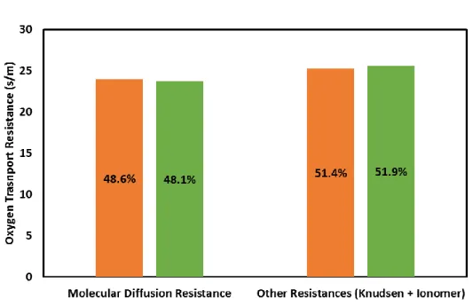
As mentioned before, the total oxygen transport resistance and the contribution of molecular diffusion resistance were obtained using the difference in limiting current density of two different inert gases. The contributions of molecular diffusion resistance are shown in Figures 12 and 13. The simulation results matched the experimental results with the maximum error of 3.3% in predicting oxygen transport contribution. Therefore, it was reasonable to presume that the model is capable of adequately estimating the oxygen transport resistance in the under-saturated condition. To further validate the model at a saturation condition, current-voltage curves were drawn and compared in the following section.
Table 7. Limiting current density results
GDL A GDL B
Diluent Gas N2 He N2 He
Experiment (A/cm2) 0.441 0.604 0.375 0.536
Simulation (A/cm2) 0.441 0.601 0.378 0.527
% Error 0.01% 0.44% 0.93% 1.63%
Figure 12. Comparison of molecular diffusion resistance and other resistances between simulation and experiment (GDL A)
Figure 13. Comparison of molecular diffusion resistance and other resistances between simulation and experiment (GDL B)
3.6. Polarization curves
Single unit cells with an active area of 25cm2 were tested to obtain polarization curves. For simulation data, a quasi-three-dimensional model was modeled to capture the spatial variation in gas composition along the channel. The polarization curves were obtained from both experiments and simulation to compare and validate the model. Figures 13 and 14 show the comparison of polarization curves between simulation and experiment of both GDLs. There were slight voltage deviations between simulation and experiment up to 0.4 A/cm2 for GDL A case. However, this error was limited to the low current density region, and it disappeared as the current density increased. Overall, the model was capable of simulating the PEM appropriately.
Table 8. Experimental condition for polarization curves
Description Value
MEA GORE PRIMEA™ 57® Series
GDL GDL A / GDL B
Active Area 25 cm2
Operating Temperature 65 ℃
Relative humidity 100 %
Inlet Gas Pure hydrogen (Anode) / Air (Cathode) Stoichiometric Ratio 1.5 (Anode) / 2 (Cathode)
Figure 14. Comparison of experimental polarization curve and simulated polarization curve (GDL A)
Figure 15. Comparison of experimental polarization curve and simulated polarization curve (GDL B)
Chapter 4. Results and Discussion
In this chapter, the individual oxygen transport resistances were obtained using the developed model. Two different GDLs with distinct physical properties were adapted to the model parameters to observe the change in specific oxygen transport resistance for each case. For operating conditions, two specific conditions were chosen. Firstly, the same condition as the previous limiting current validation was selected to further separate the empirically obtained oxygen transport resistance. Secondly, a normal air operating condition was chosen. In this case, the inlet gas was fully humidified to promote the condensation of generated water. The model simulated the oxygen transport resistance of each component even at the saturated condition.
4.1. Under-saturated condition
In the previous chapter, the total transport resistance and the contribution of molecular diffusion and Knudsen diffusion of a whole cell were empirically obtained using limiting current density. The separation of the molecular diffusion was done as a whole cell, and further separation of the transport resistance would require a number of carefully planned experiments. Fortunately, the developed model easily overcame this barrier and provided the detailed information on the oxygen transport resistance. Two sets of GDLs, namely, GDL A and GDL B were simulated to observe the change in transport resistance, and the results provided the intrinsic structural resistance on each component.
4.1.1. Limiting current density
4.1.1.1. GDL A
The oxygen transport resistance was divided into channel resistance, substrate resistance, MPL resistance and catalyst layer resistance. The catalyst layer resistance was further separated into the gas-phase diffusion catalyst layer resistance and the ionomer permeation resistance. In addition, the contribution of molecular resistance and Knudsen resistance were obtained for the MPL and the catalyst layer.
Channel-GDL interface transport resistance was 7.2 s/m, and the substrate transport resistance was 10.1 s/m. The MPL showed the highest resistance of 17.7 s/m which was consisted of 25% molecular diffusion resistance and 75% of Knudsen diffusion resistance. At the catalyst layer, molecular resistance and Knudsen resistance contributed 1.2 s/m and 4.2 s/m, respectively. Lastly, the ionomer resistance, including the oxygen permeation resistance was 8.9 s/m. Using the developed model, the total oxygen transport resistance of 49.3 s/m was divided into individual oxygen transport resistance.
Figure 16. Oxygen transport resistance of each component at under-saturated condition (GDL A)
4.1.1.2. GDL B
In a similar fashion, the model was simulated with GDL B parameter. The total oxygen transport resistance of 57.4 s/m was separated as shown in Figure 17. The channel-GDL interface resistance was the same as before, 7.2 s/m. The substrate resistance was 13.1 s/m, and the MPL resistance was 22.8 s/m. The MPL resistance was additionally divided into molecular diffusion resistance of 6.6 s/m and Knudsen diffusion resistance of 16.2 s/m. The contribution of molecular resistance and Knudsen resistance in the MPL were 29% and 71%, respectively. The resistance of the catalyst layer and the ionomer resistance were 5.4 s/m and 8.9 s/m.
Figure 17. Oxygen transport resistance of each component at under-saturated condition (GDL B)
4.1.1.3. Comparison between A and B
Total oxygen transport resistance was 49.3 s/m for GDL A, and 8.4 s/m for GDL B.
The total resistance was 8.4 s/m lower in GDL A; hence GDL A showed a 14%
reduction in oxygen transport resistance. The contribution of individual resistance for each case is shown in Figure 18 and 19.
The result indicated that MPL contributed up to 40% of the dry transport resistance.
The small scale of MPL pore size with low porosity acted as the major obstacle in oxygen transport. The MPL resistance of GDL A corresponded to 78% of GDL B.
Even though GDL A had a smaller pore size which increases the resistance, the thinner layer thickness had resulted in a smaller MPL resistance. Noticeably, the GDL A showed molecular and Knudsen diffusion resistance ratio of 1:3, while GDL B showed 1:2.46. The reason for the higher ratio of GDL A was from the smaller average pore size.
Meanwhile, channel resistances were around 12~15% of the total resistance and remained at the same resistance of 7.2 s/m. The surface roughness of GDLs influenced the mass transfer between channel and GDL. However, this effect was not considered in the model; hence the value was not changed.
Next, the diffusion in the catalyst layer was responsible for 10% of the total resistance which is a substantial amount, considering its thickness of 7 μm. Therefore, it is advised to sensibly control the water saturation in this layer to maintain the low oxygen transport resistance.
Lastly, the contribution of ionomer resistance was roughly 15%. The majority of the resistance was from the discontinuity in oxygen concentration as oxygen permeated through the ionomer.
Overall, the resistance of GDL A was lower than that of GDL B at the under-saturated condition. The reason for this outcome was derived from the higher porosity of the substrate and thinner MPL thickness, despite the smaller pore size of GDL A.
Figure 18. Contribution of individual oxygen transport resistance at under- saturated condition (GDL A)
Figure 19. Contribution of individual oxygen transport resistance at under- saturated
![Figure 1. Schematic diagram of a PEM fuel cell adapted from O’Hayre et al.[12]](https://thumb-ap.123doks.com/thumbv2/123dokinfo/11516061.0/17.808.203.619.147.520/figure-schematic-diagram-pem-fuel-cell-adapted-hayre.webp)
![Table 1. Diffusion volume of simple molecules [31]](https://thumb-ap.123doks.com/thumbv2/123dokinfo/11516061.0/28.808.132.676.827.938/table-1-diffusion-volume-of-simple-molecules-31.webp)