A Comprehensive Study of Dual Active Bridge Converter and Deep Belief Network Controller for

This dissertation presents a comprehensive study of Dual Active Bridge (DAB) converter and Deep Belief Network (DBN) controller for Bidirectional Solid State Transformers (SST). The transformer current in the DAB converter is purely alternating current, so continuous time modeling is difficult. Instead, the proposed approach uses the only 1st order terms of transformer current and capacitor voltage as state variables.

The PI gains are allowed to vary within a predetermined range and therefore eliminate problems from the conventional PI controller. The performance of the proposed AI gain scheduled PI controller is simulated and compared with the conventional fixed PI controller under steady-state error, response time and load disturbances. The DAB converter experimental system is implemented using the digital signal processing unit, Texas Instrument TMS320F28335 control board, to examine and verify the performance of the proposed controller under different operating conditions.

The simulation and experimental results show a good improvement in transient as well as steady state response of the proposed controller.

Introduction

Solid State Transformers
Candidate Circuit Configurations
Analysis and Applications of DAB Converters
Modeling of Power Converters
Control of Power Converters

A SST is able to control power flow, which is the "energy router", one of the key enabling components in the future energy system [1]. Disadvantages of the DAB converter are the high maximum value of the Root Mean Square (RMS) current through the output capacitor, the high maximum transformer RMS current through the winding, and the high complexity of the modulation algorithm that is required to generate the gate signals for generating the switches [106]. Thus, the resonant circuit of the CLLC resonant converter requires a larger volume than the inductor of the DAB converter [6].

In addition, the efficiency obtained with the DAB converter and the CLLC resonant converter is very sensitive to the ratio of the input to output voltage. This can be avoided in a two-stage arrangement that keeps the input voltage of the isolated DC-DC converter locked to nV2 [106]. The simplified reduced-order model addressed above assumes that the dynamics of the transformer current is significantly faster than that of the output capacitor voltage.

A lead-lag compensator is another type of power converter controller that increases the phase margin of the loop gain. The control design is achieved when the control input is capable of making the time derivative of the Lyapun function negative definite.

Figure 2. The Applications of Smart Solid-State Transformers [124]

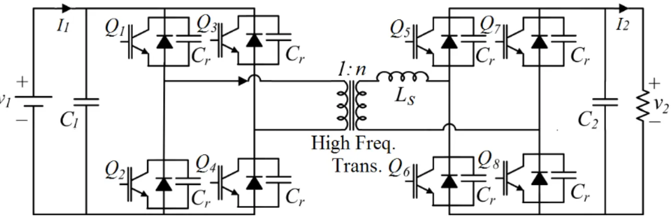
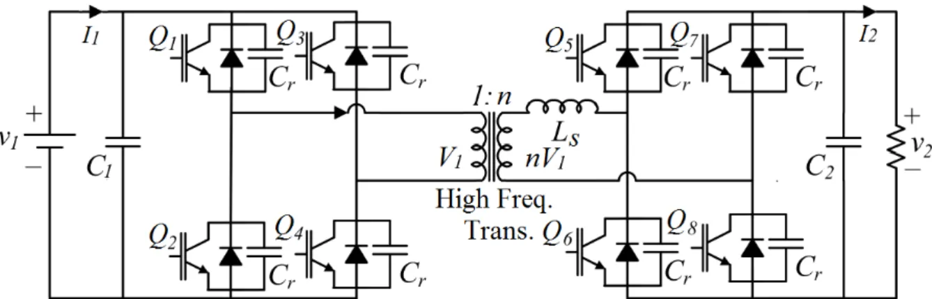
Dual Active Bridge Converters

Circuit Configuration

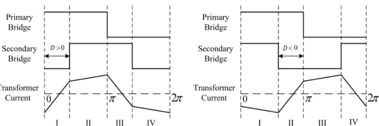
In addition, the DAB converters feature a symmetrical dual active H-bridge configuration that helps achieve bidirectional power flow. The direction and amount of power flow is regulated by controlling the phase shift between the H-bridges. Below are two modes of operation corresponding to the two directions of power flow of the DAB converter.

On the left side of Figure 8, positive power flow is defined as left-to-right power for the inverter, while on the right side of Figure 8, negative power flow is defined as right-to-left power. Positive power flow (left) and negative power flow (right) of a DAB converter The amount of power transferred to the load is controlled by the phase shift angle between the two bridges and is theoretically formulated as follows. Where V1 is the voltage of the first bridge, V2 is the voltage of the second bridge, n is the inverse ratio of the high-frequency transformer, D is the amount of phase shift between the first and second bridges, fs is the switching frequency and Ls is the leakage inductance of the transformer.

Ideally, when the converter loss is negligible, the output power is equal to the input power, and it can be shown that the voltage transfer ratio of the DC-DC DAB converter is determined by the transformer leakage inductance, the phase shift between the bridges, and the switching frequency.

Figure 8. Positive Power Flow (Left) and Negative Power Flow (Right) of DAB Converter The amount of power transferred to the load is controlled by the phase shift angle between two bridges and formulated theoretically as follow

Dual Active Bridge Converter Model

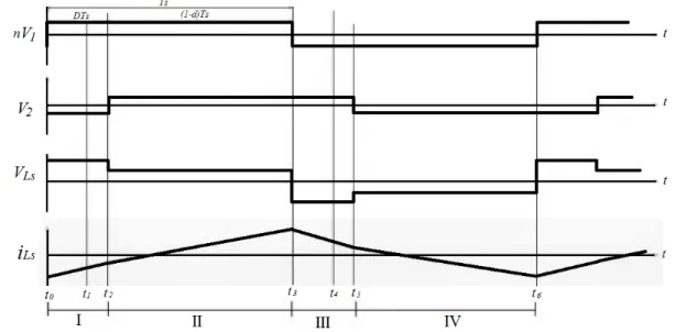
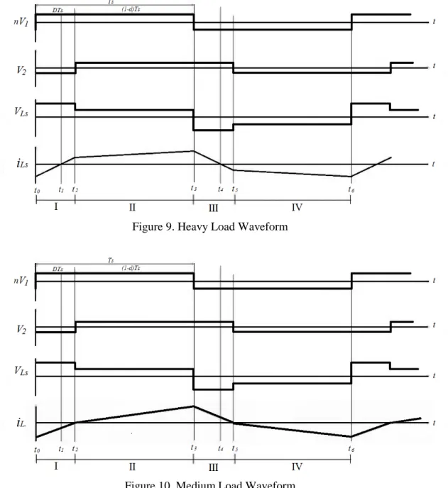
Each switching period has 6 different states and can be defined by voltage and current at each state [28, 70]. Therefore, the leakage inductor of the high-frequency transformer has a negative current, and the current on the inductor can be expressed as the following equation. The total current transition during t0 ~ t2 can be formulated and the current at t2 is derived as the following expression.

The total variation of the current during t2 ~ t3 can be displayed while defining the tracking and current. With the above whole formula defining voltage and current in each state, it may be possible to derive an equation of state as current variation. The whole state can be divided by 4 periods depending on the current variation, and a state equation can be derived to calculate an average model and a small signal model for each state period.

Finally, only first order component is considered and the others are removed, then it can be described as the following. The transfer function of system is possible to obtain using small signal model as follows [49].

Deep Belief Network Controller

Perceptrons
Feed-forward Networks
Training
Restricted Boltzmann Machines
Contrastive Divergence
Deep Belief Networks
Deep Belief Network Controller in Dual Active Bridge Converter

The training of the perceptron consists of feeding it several training samples and calculating the output for each of them. The units in the input layer serve as input to the hidden layer units, while the hidden layer units are the input to the output layer. To process input data, clamping the input vector to the input layer, setting the values of the vector as output for each of the input units.

In this particular case, the network can process a three-dimensional input vector because of the three input units. The hidden layer is where the network stores its internal abstract representation of the training data, similar to the way a human brain, greatly simplified analogy, has an internal representation of the real world. As information is sent back, the gradients essentially begin to disappear and become small relative to the weight of the networks.

The most common algorithm for supervised training of the multilayer perceptrons is known as back-propagation. As shown in Figure 22, gradient descent is universal, but in the case of neural networks this would be a graph of the training error as a function of the input parameters. Essentially, the goal is to move in the direction of the gradient in terms of weight, ie.

The key term is the derivative of the error, which is not always easy to calculate. Second, the negative phase consists of propagating h back to the visible layer with the result v', the connections between the visible and hidden layers are undirected and thus allow movement in both directions, and propagating the new v' back to the hidden layer with the activation result h. '. The input layer of the first RBM is the input layer for the whole network, and the pre-training according to the unsaturated layers works as follows.

DBN is a graphical model that learns to extract a deep hierarchical representation of the training data. Each level has a conditional distribution for the visible units that is conditional on the hidden units in the RBM, and the visible-hidden joint distribution is in the top-level RBM. At the end, each gain of the PID controller updates the new gain value according to Ku.

Simulation and Experiment

Circuit Configuration

Controller Configuration

This problem can be solved by increasing the filter order, but this is not suitable for DSP implementation due to the computational burden. However, we need to meet the minimum requirement of the statistical central limit theorem that the number of samples is at least 30. Until now, a conventional PI controller has been used, and from now on, the proposed algorithm that is an adaptive PI controller with artificial intelligence acquisition scheduling will be described as shown in the table 4.

Defining the learning rate variable is kind of a hard problem and in most cases, the learning rate starts at 0.01 is appropriate and is the most balanced point between fast and stable. Moreover, the best way to determine the learning rate is the continuous decrease from the high learning rate to the low learning rate. However, in this case, 0.1 is valid in terms of DSP, which has limited computing power for calculations.

However, there is a calculation and a time limit in this controller, so epochs are represented as the values above. Ideally, the number of hidden layers is defined as 6~7 layers or higher and the size is bell-shaped – gradually increasing and then decreasing. With these parameters, DBN predicts the conditional probabilities of the state space consisting of higher, lower or same as the reference point.

Integrating whole variable probabilities multiplied by each state variable such as -1 (going down), 0 (maintaining), 1 (going up) and then using these values it is possible to get the ultimate value of gain adjustment value Ku. Finally, we can multiply by the weight of each gain value, such as Wp, Wi, Wd, get the increase or decrease for each gain. In this kind of method, there exists a problem which is possible to occur the stability problem.

To guarantee the stability problem, truncation of the upper and the lower bound of each profit variable is a possible solution for this system. Therefore, the mean value of each gain is fixed Kp and Ki and each case is tested by bode plot as shown in Figure 32. As shown in Figure 33 and 34, the proposed algorithm needs more load as the calculation of DBN algorithm for updating PID gain variables.

Figure 31. Design Digital Filter with Matlab

Simulation and Experimental Results

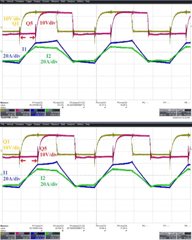
In the experiment shown in Figure 36, the amount of phase shift is slightly different, 3%, than that of the conventional PI controller at full load of 3.3 kW. It is derived from the gain variation of the PI controller, which shows that the proposed algorithm adjusts the gain value and reduces the steady state error. In the experiment shown in Figures 37, 38 and 39, the dynamics of the proposed algorithm is better than the conventional one in terms of transition state variation.

When load is changed to confirm the response transition of step load, proposed algorithm performs more stably than conventional one. In the experiment shown in Figures 40 and 41, the trend of efficiency is the lowest in light load, the highest in middle load and high in full load. The reason is that converter always consumes certain amount of energy such as switching loss, conduction loss, heat and sound and free running current.

Figure 36. Conventional (Top) and Proposed (Bottom) Full Load 3.3kW Waveform

Discussion and Conclusion

Future Work