Orientation measurement system is required to improve orientation control by sensing the orientation of an object. This thesis presents to develop an orientation measurement system that uses magnetic field of permanent magnet and magnetic sensors such as Hall effect sensor. Using the magnetic field of a permanent magnet, the orientation of an object embedded with these magnetic sources can be detected in real time.
The magnetic field-based orientation tracking method has advantages such as non-contact measurement without any additional mechanics and no requirement for the line-of-sight problem. However, due to the complexity of the relationship between the magnetic field and the position/orientation, it is challenging to calculate the position/orientation from the closed-form magnetic field. Using the distributed multipole model which can provide a fast and closed form to analyze the magnetic field, issues related to this system are studied including the optimized sensor number and sensor position.
In both the simulation and the experiment, two examples are introduced to better understand how the proposed measurement system can measure orientation and evaluate a measurement accuracy according to a motion area, considering problems. Rji±- Distance vectors of source and sink from the ith dipole in the jth loop to a sensor position.
INTRODUCTION
- Background and Motivation
- Prior and Related Works
- Research Objective
- Thesis Outline
Lee and Son developed a method to obtain orientation from magnetic field inverse by using a combination of sine and cosine function [16]. Since the relationship between magnetic field and orientation has periodic patterns, the function defining the relationship can be represented by a combination of sine and cosine. Son and Guo have been proposed to use the magnetic field measurements of permanent magnets in moving rotors (PMs) and ANN [17].
In a magnetic field based position/orientation measurement system, another critical issue is the one-to-one mapping between the orientation of the PM and the magnetic field (=bijective relationship). The aim of this research is to develop an orientation measurement system using a PM magnetic field and magnetic sensors such as a Hall sensor. By using the PM magnetic field, the orientation of the object embedded with this magnetic source can be monitored in real time.
When the PM moves, a static magnetic field is established in the movement area and can be calculated by the DMP method. Algorithms for obtaining orientation from magnetic field with artificial neural network are introduced and issues related to this system are studied.
TWO-DOF ORIENTATION MEASUREMENT SYSTEM
Overview
This method can provide a quick and closed solution against which other methods such as ANSYS or analysis are compared. The MFD calculated by DMP is used to study the problems with this system. Two examples are introduced to validate that the proposed method can measure the orientation in numerical simulation and experiments.
Using only a single sensor identifies how much orientation can be measured in a range of motion. Based on the result of Example 1 using single sensor, the multi-sensor approach is used to expand a sensing area and reduce measurement error.
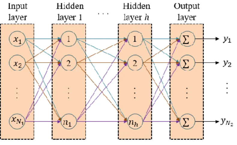
Orientation Measurement System based on Magnetic Field and Artificial Neural Network
- Magnetic field of Permanent Magnet Based on DMP
- Analysis of Bijective Domain
- Investigation of Optimized Sensor’s Position and Orientation
- Measurement Accuracy based on Jacobian matrix
- Inverse Computation by using Artificial Neural Network
- Multi-Sensor Approach
- Calibration of Magnetic Field
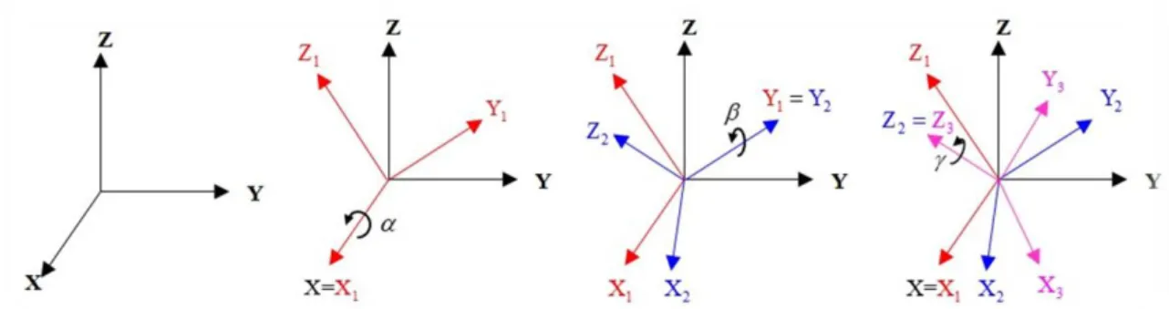
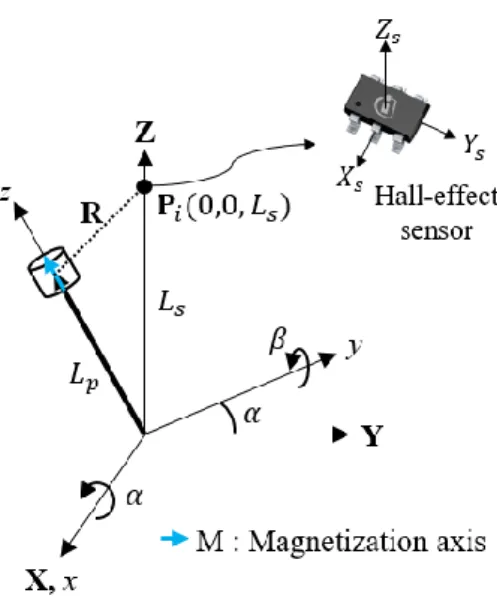
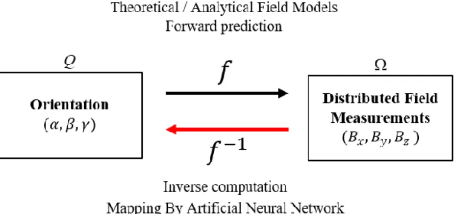
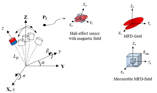
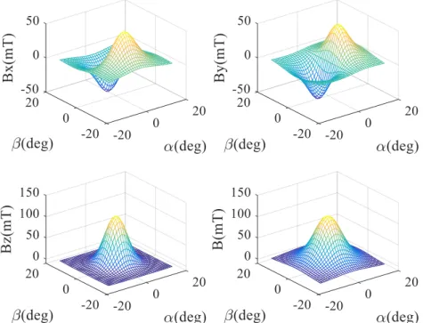
The orientation of PM can be defined as , and γ, which are the rotation angles about the X-axis, y′. Due to the symmetry of the magnetization of PM along the z-axis, only two Euler angles ( and in Figure 2.3) can be measured. The MFD can be calculated with given posture using theoretical/analytical field models (=Forward prediction).
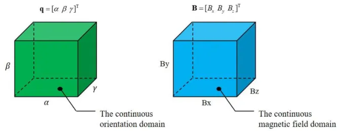
The mutual relationship can be determined using simulated MFD and orientation. The continuous domain of orientation and MFD can be visually illustrated in Figure 2.6 [19]. Since the continuous domain of MFD and orientation are decretized by DMP, the bijective domain can be determined numerically. If the dimension of MFD is much larger than the orientation, the left inverse should be applied in Eq. (2.10) and the determinant of the former term can be calculated because it is a square matrix.
Similarly, the orientation dimension is much larger than MFD; the right inverse should be applied in equation (2.11). The MFD field can be formed by the orientation of PM and the position of a sensor, assuming that the rest of the parameters are determined based on the system design. In the spherical shape of a measurable MFD field, the magnitude of the MFD is smaller than the maximum value and larger than the minimum value in Eq. (2.12).
In the quadratic form of the MFD measurable field, the absolute MFD is less than the maximum value and greater than the minimum value of each axis in equation (2.13). Equation (2.15) shows that the change of the magnetic field with respect to the desired angular resolution must be greater than the resolution of the used magnetic sensor. The optimized sensor position and orientation for a given magnetic sensor can be achieved by maximizing the sensing performance in Equation (2.16).
The root-mean-square error (RMSE) is the cost function that attempts to minimize the square root of the squared error between the output of the ANN and the desired target in Eq (2.22). For practical simulation, the magnetic field variation and uncertainty included in the simulated MFD in Eq. (2.25). In numerical simulation, the MFD variation model in Eq (2.25) is used to identify the measurement accuracy according to a range of motion.
Numerical Simulation and Experiment
- Example 1: Two-DOF Orientation Measurement System with Single Sensor
- Example 2: Two-DOF Orientation Measurement System with Multi-Sensor
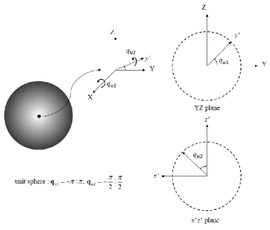
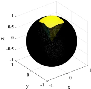
The unit sphere in figure 2.9 can be applied to this system to identify the sensor performance, because the two constraints in equation (2.17) and (2.18) are satisfied. Pi is set as [0 0 Ls=83]T. The colored area is the area that satisfies both conditions and the black sphere is the unit sphere. In Figure 2.15 (a) and (b), the empty area appears in the center of AC12u because the narrow distance between the PM and the sensor is causing saturation of the sensor.
B (=[Bx By B]T) are used for the ANN, since the area satisfying the bijective relationship between q and [Bx By B]T is larger than [Bx By Bz]T, as shown in Figure 2.17 ( d). Two conditions in equations (2.5) and (2.6) are satisfied, as B and q are uniquely determined without overlap, as shown in Figure 2.18 (a). In view of this problem, the measuring points of the sensor are calibrated using the XYZ phase, shown in Figure 2.22 (a), before the Hall effect sensor is applied to the measuring system.
It is possible to find the center of the yz plane by checking that the value of By and Bz are zero simultaneously as shown in Figure 2.22 (b). Similarly, the center of xz plane can be found by checking that the value of Bx is Bz is zero simultaneously as shown in Figure 2.22 (c). Maximum adjustment ranges for each step are respectively ±15° and ±20° indicated in product information as shown in Figure 2.24.
The first column of Figure 2.25 shows the weight and bias of each axis according to the number of actual measurements Ns and the second column of Figure 2.25 is the MFD calibration error between the simulated MFD and the actual measurements. The magnetic field distribution discretized by the DMP of each sensor is the same in Figure 2.13, but the orientation region differs. The center of the orientation region in Figure 2.13 was set as qs=[0 0]T because the magnetic sensor of example 1 is at the initial position of the sensor.
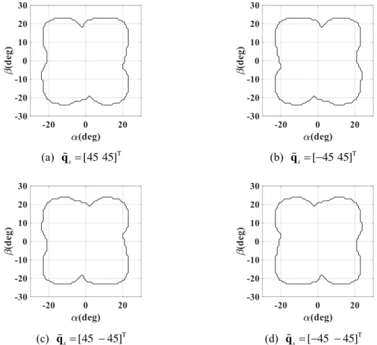
With this characteristic of the bijective domain, the measurement error of each closed circle could be identified in Figure 2.28 and Table 2.6. A closed circle can be approximated to a closed square with length ac=rc×cos45°×2 of one side as shown in Fig. 2.30 (a). Thus, a closed square with the desired precision can be used to extend the detection area, as shown in Figure 2.30 (b).
On the contrary, if m is the oven number, the sensors are connected together without the sensor, where the position is in the initial sensor position, as shown in Figure 2.30 (b). The red and blue solid lines in Figure 2.33 are the actual measurements and the calibrated MFD by applying weight and bias respectively.
Conclusion
CONCLUSION AND FUTURE WORKS
Accomplishments and Contributions
Future Works
Lee, “Nonlinear compensation of a novel non-contact lever using universal joint mechanism,” IEEE/ASME Trans on Mechatronics, vol. Stein, "Kinematic Design and Switching of a Spherical Stepper Motor," IEEE/ASME Trans on Mechatronics, vol. Son, “Distributed multipole model for the design of permanent magnet-based actuators,” IEEE/ASME Trans on Magnetics, vol.
Chen, “A robust adaptive iterative learning control for trajectory tracking of permanent-magnet spherical actuator” IEEE Trans op Industrial Electronics, vol. Hollis, "Initial results for a ballbot driven with a spherical induction motor," IEEE International Conference on Robotics and Automation (ICRA), Stockholm, Sweden, pp. Lee, "Open-loop controller design and dynamic characteristics of a spherical wheel motor," IEEE Trans on Industrial Electronics, vol.57, no.10, pp.
Espi’e, “Mechatronics, Design and Modeling of a Motorcycle Driving Simulator,” IEEE/ASME Trans on Mechatronics, vol. Zhou, “A real-time optical sensor for simultaneous three-DOF motion measurement,” IEEE/ASME Trans on Mechatronics, vol. Lee, “Design and Analysis of an Absolute Contactless Orientation Sensor for Wrist Motion Control,” IEEE/ASME International Conference on Advanced Intelligent Mechatronics (AIM), p.
Chan, “A linear algorithm for magnet position and orientation tracking using 3-axis magnetic sensors,” IEEE Trans on Magnetics, vol. 43, no. Son, "Design of a sensing system for a spherical motor based on hall effect sensors and neural networks," IEEE International Conference on Advanced Intelligent Mechatronics (AIM), Busan, Korea, p. Bai, “Harnessing embedded magnetic fields for angular sensing with nanoscale precision,” IEEE/ASME Trans on Mechatronics, vol.
Bai, “Direct field feedback control of a ball-joint-like permanent-magnet spherical motor,” IEEE/ASME Trans on Mechatronics, vol. Leonovich, "A new method for magnetic position and orientation tracking," IEEE/ASME Trans on Magnetics, pp. Fang, “Optimization of measuring magnetic fields for position and orientation tracking,” IEEE/ASME Trans on Mechatronics, vol.
![Figure 2.18 shows the MFD domain of B (=[B x B y B] T ) and the narrow parts with orienatation domain](https://thumb-ap.123doks.com/thumbv2/123dokinfo/10522676.0/41.892.273.594.147.464/figure-shows-mfd-domain-narrow-parts-orienatation-domain.webp)
