In this thesis, several efficient numerical methods are proposed to solve initial value problems and boundary value problems of fractional differential equations. For problems with fractional initial values, we propose a new type of predictor-evaluate-corrector-evaluate method based on the Caputo fractional derivative operator. Furthermore, we propose a new type of the Caputo fractional derivative operator that does not have a differential form of a solution.
For partial GDPs, we propose an explicit method that dramatically reduces the computational time for solving the dense matrix system. In addition, by adopting high-order predictor-corrector methods that have uniform convergence rates of O(h2) or O(h3) for all partial orders [8], we propose a second-order method and a third-order method using Newton's method and Halley's method, respectively. From this the field of fractional calculus was born and several well-known definitions of fractional integral and derivative were developed, such as Riemann-Liouville operators, Caputo operators, Hadamard operatos and Gr¨unwald-Letnik derivative. .
Moreover, due to the non-local properties of a partial derivative, there are still many improvements to the conventional numerical approaches for solving di↵ fractional equations in terms of computational algorithms. First of all, we propose a new type of numerical method for solving fractional IVPs: the direct method. To reduce the computational cost, we propose the high-order method that changes a BVP into an IVP and use the nonlinear firing method for updating an approximation of an IVP.
Then, the new scheme achieves a uniform order of accuracy regardless of the fractional order value by adopting a modified PECE method [8], Newton's Method, and Halley's Method.
Preliminaries
There are several well-known definitions that define fractional derivatives, such as the Caputo operators, the Riemann-Liouville operators and the Gr¨unwald-Letnikov definition. However, we are interested in the Caputo fractional operator, which is an alternative operator to the Riemann-Liouville fractional differential operator. The most important point is that they do not generally coincide and the following is not the left-inverse operator of the Riemann-Liouville fractional integral operator.
R is continuous and bounded in G and that it satisfies the Lipschitz condition with respect to the other.
Conventional Numerical Methods for Solving FDEs
- Description of Direct Method
- Direct Method with Linear Interpolation
- Direct Method with Quadratic Interpolation
- Error Analysis
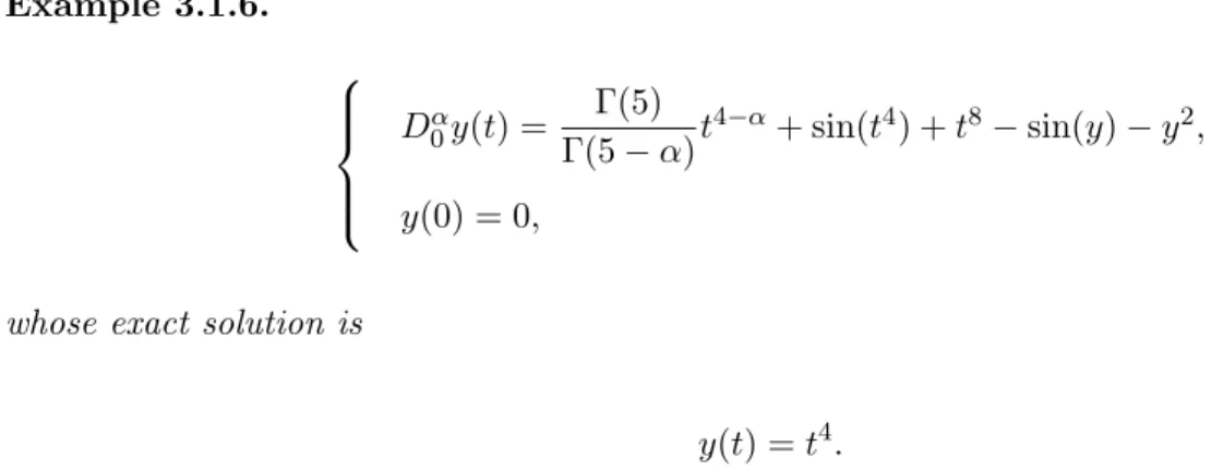
- Numerical Examples
Then we can solve the fractional differential equation by updating only a numerical solution on a current interval. To solve the problem numerically, we use a fractional derivative in the Caputo sense (2.1.5), i.e. t s)m 1 ↵y(m)(s)ds, (3.2) because it imposes the initial conditions with homogeneous conditions . In conventional methods based on Caputo's fractional derivative, the derivative of a solution is approximated by linear interpolation or quadratic interpolation.
In terms of numerical approaches, the main difficulty to tackle is the non-locality property that the solution(t) has due to the kernel (t s)↵ 1 under the integral equation on the right-hand side of Eq. On (tn 1, tn) the integral can be simplified with Z tn. 3.11) Therefore, ˜yn can be evaluated by solving the following equation. Furthermore, the first two terms on the left-hand side of (3.12) can be simplified by
In this section we further improve our scheme by applying a quadratic interpolation of y(t) over each interval Ij = [tj, tj+1]. Now the value off(tn, y(tn)) can be approximated using the quadratic interpolation off(t, y(t)) with grid points tn 3, tn 2 and tn 1. 3.7), where the uniform property of the grid, that's what we get. 3.19). Leten=y(tn) could be an error at time steptn. Truncation error with linear I-interpolation) Let ⌧n be a truncation error on tn.
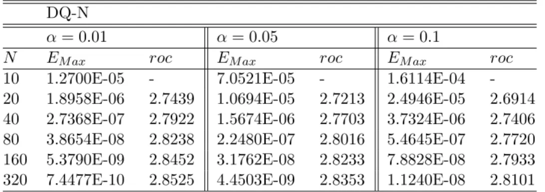
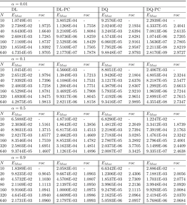
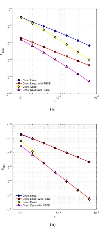
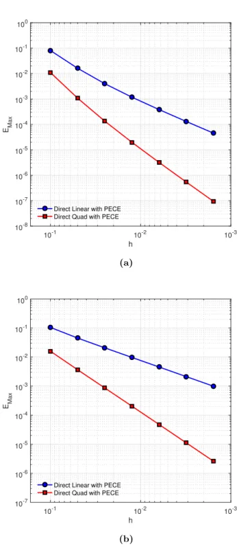
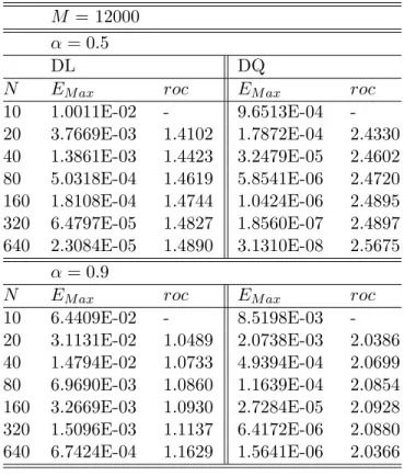
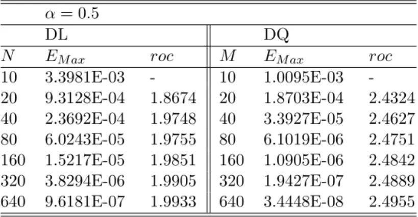
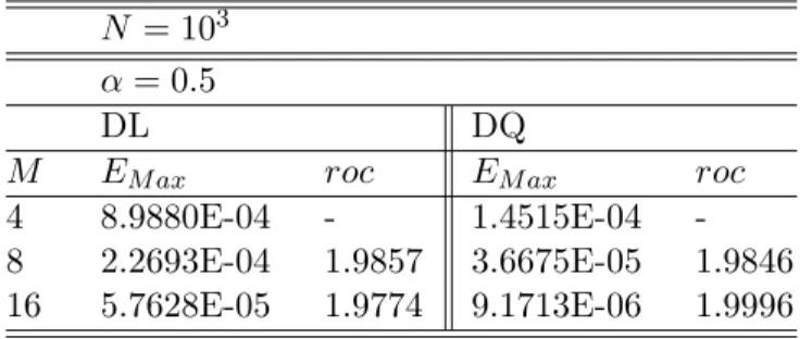
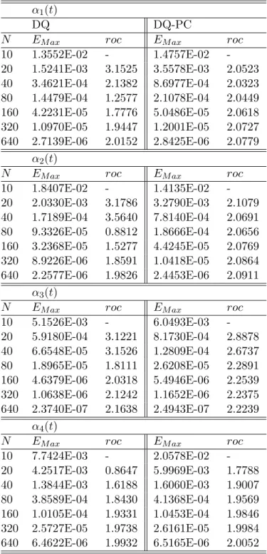
By a similar procedure in theorem (3.1.3), we can obtain the analysis for the order of accuracy of the new scheme using a quadratic interpolation. Truncation error with quadratic interpolation) Let ⌧n be a truncation error at tn. Following similar procedures in Theorem 3.1.3, we obtain the truncation error for the quadratic interpolation. In this section, we illustrate the accuracy and efficiency of our new methods, both with linear (DL) and quadratic interpolation (DQ).
Let N(⌧) be a number of steps (a step size) in time and M(h) be a number of steps (a step size) in space. Then we can expect a global convergence with O(h2) andO(⌧3 ↵) by checking each step size for linear and quadratic interpolation respectively. By definition 3.1.1, we can solve an IVP of variable fractional order using our numerical methods.
Enhanced Direct Method
- Newton’s Method for ↵ ⇡ 0
- Decomposition Method for ↵ ⇡ 1
- Numerical Examples
- Description of High-Order Method
- Second-Order Scheme with Newton’s Method
- Third-Order Method with Halley’s Method
- Error Analysis
- Numerical Examples
We have a stability problem in the previous method, but the problem is eliminated by combining with Newton's method. But since Newton's method is for an integer order system, we need to adjust it for a fractional system to update an approximation. When we update an approximate solution yb(T), we can apply it by Newton's method until F(s) becomes small enough.
By using Newton's method with high-order methods to solve the FDE, we have limitations in obtaining an accurate approximate solution. Newton's method has second-order convergence and the initial condition must be close enough to the exact value. So, even if we use the high-order method to solve the FDE, which has higher convergence than the second-order method, we do not expect any improvement in terms of using the high-order method with Newton's method.
It is clearly shown in the error analysis of our method with Newton's method. Suppose we can get the value(s) at t=T using a shooting method with Newton's method in a fixed interval [a, T] with an initial value s0. Then the high-order method with Newton's method has a convergence speed of at least 2nd order, where 2 = min{2, 1}.
In the direct method, we proposed a new type of Caputo di↵ercial operator without a derivative using integration by parts. For a small fractional order, we proposed the extended direct method with Newton's method for a stable numerical solution. In the high-order method, we change a BVP to an IVP instead of solving a matrix system which causes a lot of computational time.
In terms of computational mathematics, we can expect tremendous improvements in the use of our explicit methods. 8] Thien Binh Nguyen and Bongsoo Jang, A high-order predictor-corrector method for solving fractional order nonlinear di↵differential equations, Fractional Calculus and Applied Analysis no. He always guided me and helped me to continue on the right path both academically and personally.
I would also like to thank many other professors, my lab mates and other members in the department of mathematical sciences. Even though I am now starting a new journey in the US, I will always remember all the support I have back in Korea.