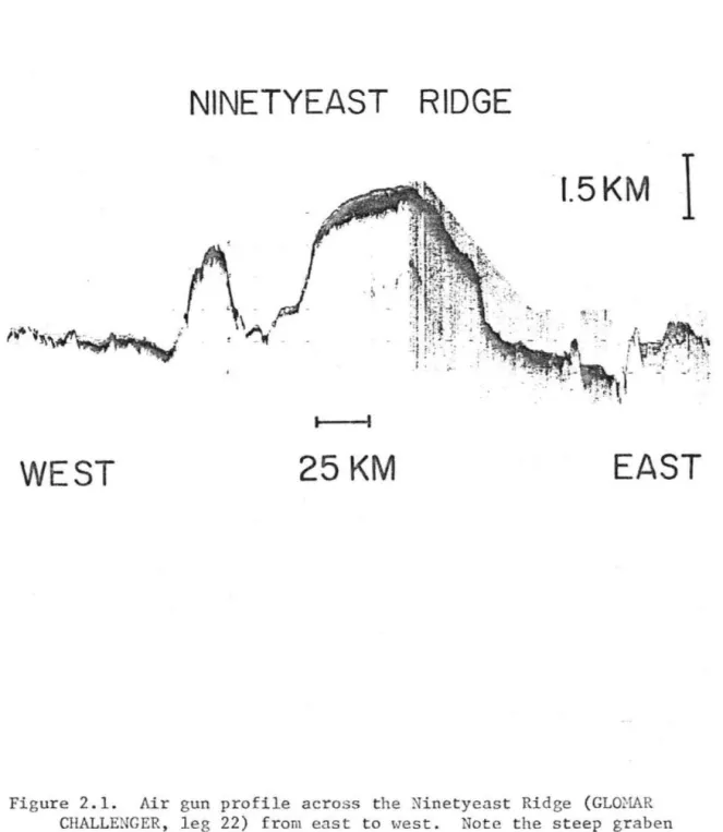
Okal, Seismicity and tectonics of the Ninetyeast Ridge area: Evidence for internal deformation of the Indian plate, J. Test of the ridge (and south of 7°S) reveals a complex terrain consisting of northeast ridges and deep, along with a broad bathymetric high (15°5, 87°E) named Osborne Knoll by Sclater and Fisher [1974].
NINETYEAST RIDGE
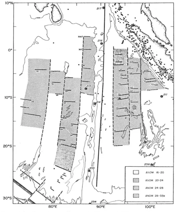
ImJ ANOM 24-28
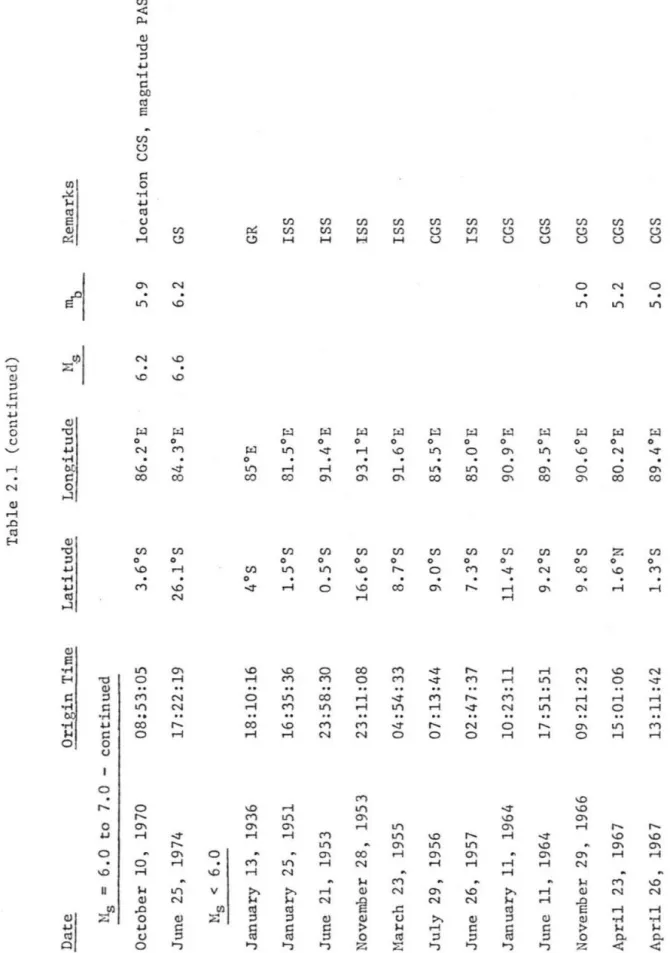
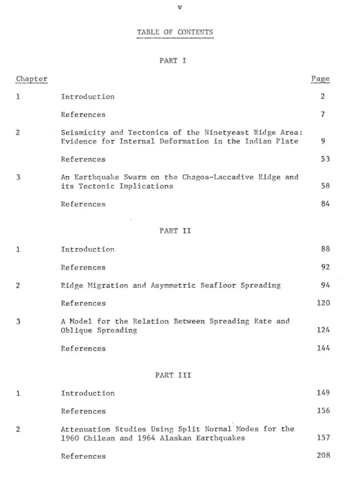
Seismicity of the Ninetyeast Ridge area (Table 2.1) plotted on the bathymetric map of Sclater and Fisher [1974]. Five of the largest earthquakes in the area (three magnitude 7 and two magnitude 6) have been relocated for various reasons.
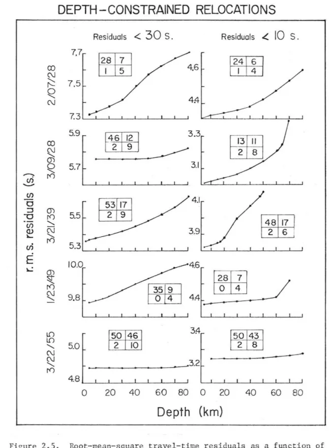
DEPTH - CONSTRAINED RELOCATIONS
Depth (km)
For t,;o of the older events, a small fraction of the stations reported first motions, as well as times, to the ISS. Given these difficulties and the small number of stations reporting, only one aircraft could be reliably limited from the initial movements.
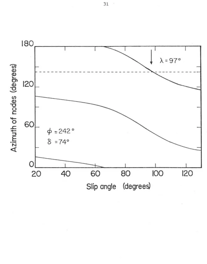
Slip angle (degree!:J
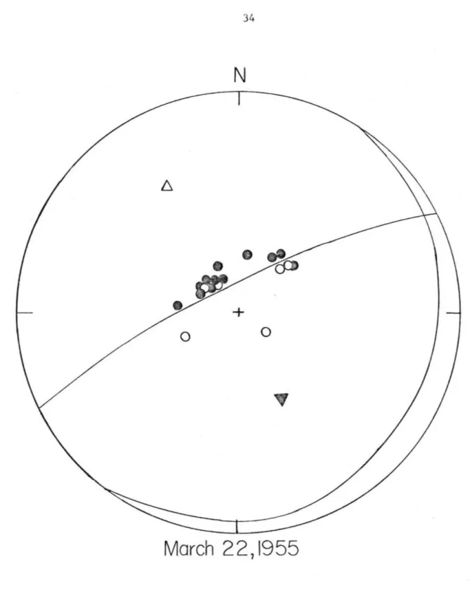
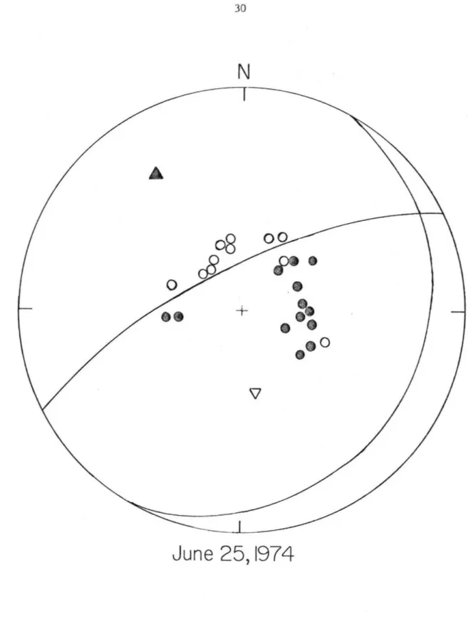
March 22 ,1955
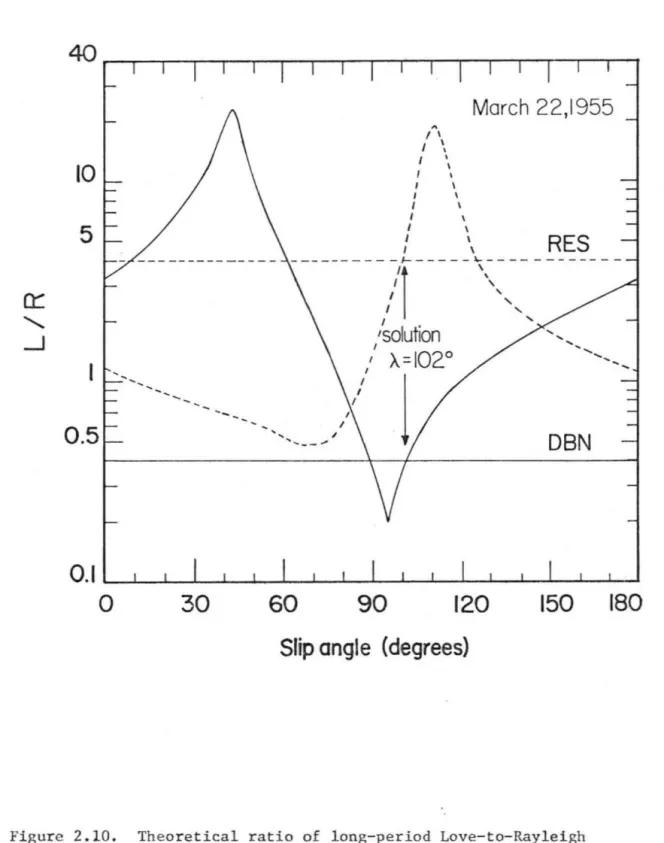
Slip angle (degree s)
March 21 .1939
This is consistent with the ridge width and general N-S direction of seismicity and concns. Chase [1978) addresses this problem using the opening of the African rift, while Minster and Jordan [1978) favor internal deformation of the Indian plate.
VEMA F.Z
Fault zone, across the eastern foot of the Central Indian Ridge, to the Chagos Bank Ridge [Fisher et al., 1974]. 1971] suggested that as the Central Indian Ridge formed, spreading ripped apart the Hascarene and Chagos Plateaus. Bathymetry shows that if the Nascarena Plateau and the Chagos-Laccadiva Ridge are rotated back together, the Chagos Bank fits between the banks of Saya de Nalha and Nazareth.
This model for the evolution of the Chagos-Laccadive and Central Indian Ridge, as well as the Nascarene Plateau is shown in Figure 3.3.
CHAGOS-
RIDGE
RECO NST RUCT ION
C PRESE NT
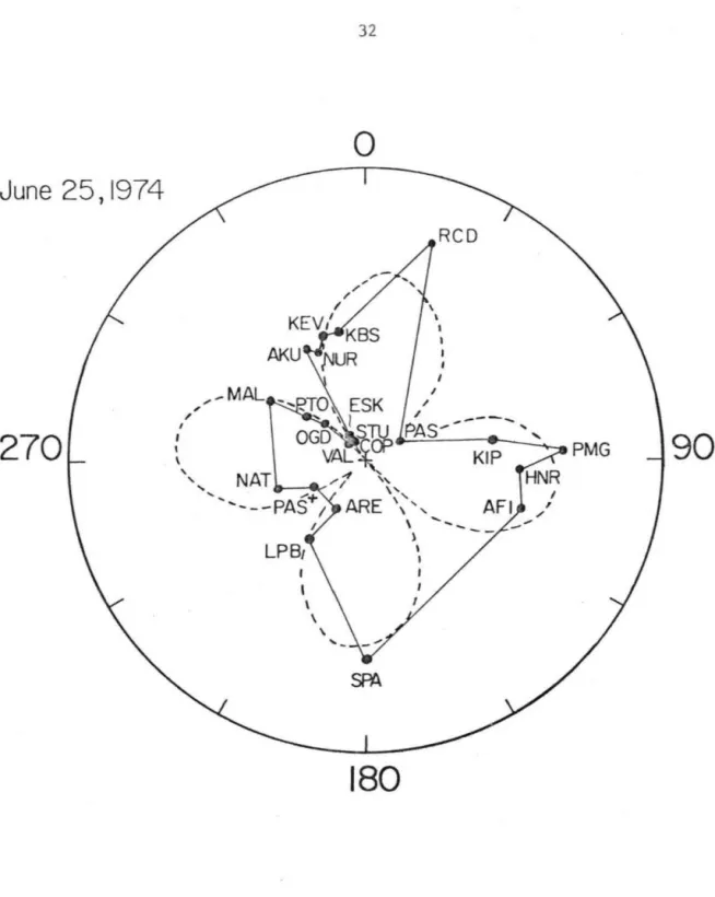
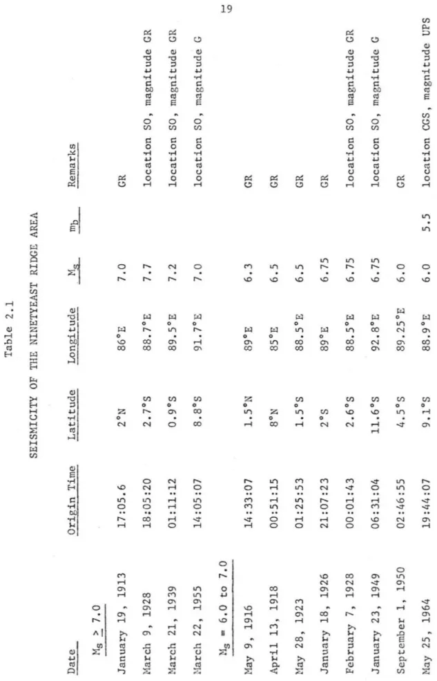
Station coverage is good for the largest event, and poorer for the two smaller events. The spectral density averaged over the 30-40 second period band is plotted for the two smaller ones. All three events represent normal faults at a substantially eastern, 'highest level, as summarized in Table 3.2. Banghar and Sykes [1969], using first motions and S-wave angles, proposed a solution for the 1965. event with a much larger component of strike-slip motion.
What a . solution is not compatible with the surface "aves.. proposed mechanisms for the other t1;.,tO events,consistent with these solutions.
GROUP VELOCIT
KM/SEC
70 PERIOD
90 SECONDS
2226 ARRIVAL
2277 SECONDS
The scaling relations of Geller [1976J suggest that an earthquake of Hs 6.0 would have a moment of 8 x 1024 dyne-cm, almost an order of magnitude less than determined from the surface waves. Such an anomalous high moment was also noted from the Oroville earthquake by Hart et al. [1977J.). Following Fukao [1971J and Kanamori and Stewart [1976J], the problem can be simplified by replacing all nearby source structures with a homogeneous layer.
These simplifications are only valid for the first few seconds of the body wave seismogram.
LEM MAL MUN NAI WIN AAE
20SEC SEPTEMBER 12, 1965
Francis and Shor, 1966] was used for the calculations.) The focusing mechanism (Figure 3.5) indicates that all but a few near-nodes all Indian stations are in the dilational quadrants, in which the waveforms vary only slightly with azimuth . For a focal depth of 15 km, the data and the synthetic data agree well for 10-12 seconds, until additional body wave arrivals appear on the plate. The source-time function, a symmetrical three-second trapezoid with a one-second rise time, yielded the best fit of any tested variety.
Such a discrepancy, suggesting that the source had a significant long‐period component, has been reported for other events, including the Oroville earthquake [ Hart et al ., 1977 ].
SEPTEMBER
IS T NDI
NHA AAE
Its location on the steep slope of the Chagos Bank is not easily explained by conventional tectonic models. Thus, the shoal cannot be easily correlated with any of the bathymetric features of the area. A still-active fracture at depth, left over from the breakup of the Chagos Bank and Nascarene Plateau, offers a possible explanation for this unusual swarm.
Fisher, Development of the east-central Indian Ocean, with emphasis on the Ninetyeast Ridge tectonic setting, Geol.
PART II
1959] reported prominent axial rifting running the length of the mid-Atlantic Ridge, "hile Menard [1960] showed that the East Pacific Rise had, instead, an axial high. Excellent overview of early developments in the understanding of Midocean ridges are provided by Wertenbaker [1974] and Uyeda [1978] After seafloor spreading "as established, the mechanics of the process became a major topic of study.
Simple geometric considerations (for example, the fact that Antarctica is surrounded by ridges) showed that ridges migrate with time.
FZB I
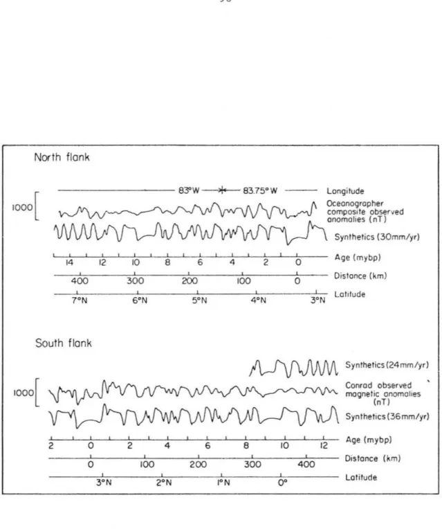
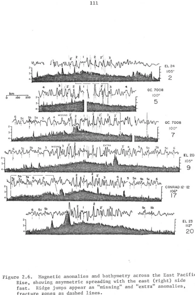
The first analyzes of seabed magnetic anomalies placed great emphasis on the striking symmetry of the profiles around the ridge. The position of the ridge axis therefore controls the difference of the two half spreading rates even though their sum is fixed. This can be used to identify the trailing flank of the ridge and predict the direction of asymmetric spreading.
Consider a reference frame attached to the reef, and a region of the crust and upper mantle that encloses it.
Slow Fast
Note that V is the relative velocity of the t,w plates: it is independent of the velocity of the plates or the edge ', with respect to the deep mantle. A positive asymmetry A indicates that the posterior flank of the ridge is spreading most rapidly, as illustrated in Figure 2.1. 34;e described does not involve thermal disturbances on either flank of the edge. These are only affected by the different spreading rates.
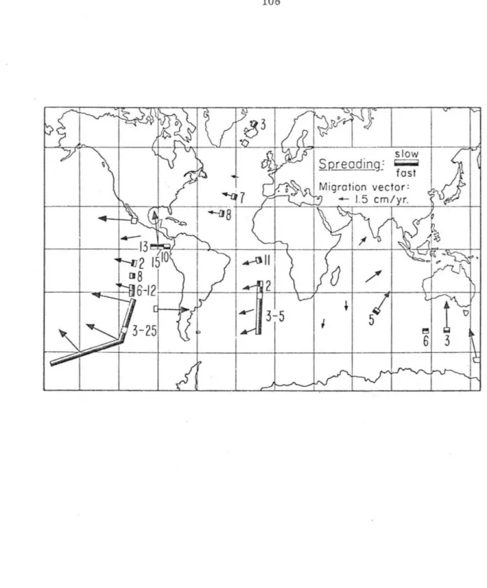
The arrows point in the direction of migration of the edge relative to the deep mantle (assuming it is trapped in the hotspot frame) and have lengths proportional to the migration rate. For convenience, the migration vectors are calculated negligibly. the small correction factor Va' which is always much smaller than the total spreading quantity.
FRACTURE
ZONE
TIME SCALE
Often the distribution is symmetric, but this model predicts a preferred direction of asymmetric distribution rather than its certain occurrence. Some of this variation may be due to noise in the data, but it still appears that the magnitude of the asymmetry is controlled by local effects. The full complexity of the process of asymmetric spreading can be seen in detailed studies of the FAl'IOUS area [Macdonald, 1977; Hacdonald and Luyendyk , 1977 ].
Clearly, no simple model of reef dynamics can adequately describe these local effects.
COCOS
NAZCA
1977] suggest that asymmetric spreading at the Galapagos Ridge is associated with the hotspot to the south. Thus, the Costa Rican rift may be far enough away to be unaffected by any outflow from the hotspot. This model is based on their observation that bathymetric data south of Australia ShOl, depths on the southern (Antarctic) flank of the ridge are consistently shallower.
Trehus's [1975] study of the South Pacific and Galapagos ridges shows that on both ridges the bathymetric.
The direction of the observed asymmetry appears to be that predicted by considerations of ridge mechanics and. Luyendyk, Deep-tow studies of ridge structure Hid-Atlantic ridge Crest hear 37°N (F"~'1OUS), Geol. Simple ridge models and transformation shm' that the minin:um energy dissipation configuration is a function of scattering rate.
Lonsdale [19771>] proposed that this orthogonality was characteristic of the rapidly spreading East Pacific Rise.
![Figure 3.1. Side-looking sonar map of the Kurchatov Fracture Zone area [Searle and Laughton, 1977]](https://thumb-ap.123doks.com/thumbv2/123dok/10413548.0/132.869.86.791.77.1006/figure-looking-sonar-kurchatov-fracture-zone-searle-laughton.webp)
OBLIQUE ANGLE
Thus, the trend of the ridge transform system determines the upper limit of oblique spreading. The present system of ridges and re-forms apparently often has enough local trend for all. . for some oblique propagation. This is consistent with Hith's minimum energy idea and suggests that for 101; rate of expansion, the ratio of transformation energy dissipation to ridge energy dissipation increases slightly.
These curves are drawn with FAHOUS data as a fixed point, as these are probably the best cjata.
II OBLIQUE SPREADING
This may be partly due to local variations in the angle B which controls the rr.aksimum skew distribution. This section presents t«o simple models of a transform error, showing a dependence on the pot. ;er on the spreading rate vanishes. The diffusion rate dependence differs between the two models, and its effects can be contrasted.
However, Figure 3.5 shows that the rate of work performed on the transform depends on the distribution rate.
Thus, for a shear stress of' pmver distributed per unit length in the fault is. POL,er has an additional rate of propagation factor because the viscous stress depends on the strain rate. C., ~ear lower magnetic anomaly, asymmetric spreading, oblique spreading, and accreting plate boundary tectonics at the Hid-Atlantic Ridge near 37°:-1, GeoI.
Luyendyk, Deep-to' studies of the structure of the Mid-Atlantic ridge near 37°N (BERETT), Geol.
PART III
Following the observation of split peaks with varying amplitudes in the free oscillation spectra of the 1960 Chilean earthquake [by Ness ~~., 1961 and Benioff Pekeris ~ al. It is therefore not possible to measure Q using the amplitude of the beat pattern as a function of time without determining the amplitude and phase of the individual oscillators. I t is based on the results of Stein and Geller [1977) for the theoretical amplitude and phase of the single tracks excited by an earthquake source of knmm fault geometry.
The results of a later analysis by Smith (1961) of the spectrum differed slightly, but did not change the situation.
DOUBLE COUPLE
C SOURCE
DOUBLE COUPLE ISOTROPIC SOURCE
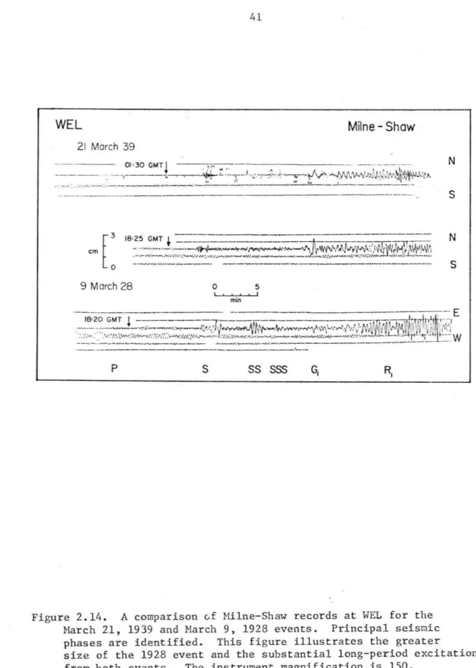
Data and synthetic data for OS2' The top trace consists of filtered data from the high-permeability Isabella strain record of the Chilean earthquake. This makes it possible to describe the complex time series resulting from the interference of the singlets. In addition, the long (500 hour) UCLA gravity gauge record is used to estimate the Q of the longest period radial mode.
To transform the excitation coefficients from the source coordinates to the geographic coordinates, use the rotation matrix elements.
NETWORK STRAIN
TIDES REMOVED
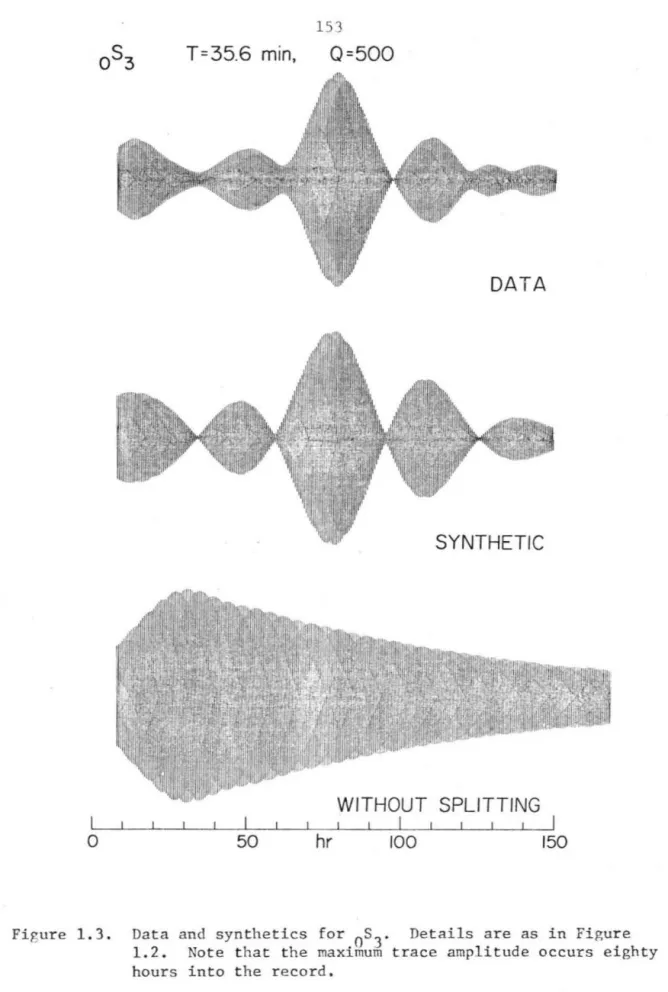
Dahlen [personal communication1 states that more accurate recent calculations show this. the elliptic splitting parameters of the spheroidal mode can be neglected for our purposes. Data and Synthetics for OS3' The noise level is one digital unit and the smoothing window is 100 hours long. Data and Synthetics for OS4' The noise level is one digital unit and the smoothing window is SO hours long.
Data and synthetic for OT4' The noise level is one digital unit and the smoothing window is 30 hours long.
![,s, oS.. oSo0S5 oT] Of4 Figure 2.4.](https://thumb-ap.123doks.com/thumbv2/123dok/10413548.0/175.879.99.787.85.1029/s-os-oso0s5-ot-of4-figure-2-4.webp)