저작자표시-비영리-변경금지 2.0 대한민국 이용자는 아래의 조건을 따르는 경우에 한하여 자유롭게
l 이 저작물을 복제, 배포, 전송, 전시, 공연 및 방송할 수 있습니다. 다음과 같은 조건을 따라야 합니다:
l 귀하는, 이 저작물의 재이용이나 배포의 경우, 이 저작물에 적용된 이용허락조건 을 명확하게 나타내어야 합니다.
l 저작권자로부터 별도의 허가를 받으면 이러한 조건들은 적용되지 않습니다.
저작권법에 따른 이용자의 권리는 위의 내용에 의하여 영향을 받지 않습니다. 이것은 이용허락규약(Legal Code)을 이해하기 쉽게 요약한 것입니다.
Disclaimer
저작자표시. 귀하는 원저작자를 표시하여야 합니다.
비영리. 귀하는 이 저작물을 영리 목적으로 이용할 수 없습니다.
변경금지. 귀하는 이 저작물을 개작, 변형 또는 가공할 수 없습니다.
Master's Thesis
Remote Influences of ENSO and IOD on the Interannual Variability of the West Antarctic Sea Ice
Jihae Kim
Department of Urban and Environmental Engineering (Environmental Science and Engineering)
Ulsan National Institute of Science and Technology 2021
[UCI]I804:31001-200000372528 [UCI]I804:31001-200000372528
Remote Influences of ENSO and IOD on the Interannual Variability of the West Antarctic Sea Ice
Jihae Kim
Department of Urban and Environmental Engineering (Environmental Science and Engineering)
Ulsan National Institute of Science and Technology
i 1
ii
ABSTRACT
2 3
This study focused on remote influences of El Niño–Southern Oscillation (ENSO) and Indian Ocean 4
dipole (IOD) on the interannual variability of the West Antarctic sea ice. The sea ice of the West 5
Antarctic has a large variability and is linked to tropical conditions such as ENSO and IOD. The sea ice 6
of the Antarctic is important. According to previous studies, the sea ice extent of the Antarctic is 20%
7
greater than in the Arctic, thus could result in dramatic changes to planetary albedo. Also, feedbacks 8
sea ice change and ocean temperature and salinity play a role in determining the stability of Antarctica’s 9
massive ice shelves and its melting directly associated with global sea-level-rise. ENSO and IOD are 10
well known phenomena that impact on the Antarctic sea ice, but which one has a higher impact is not 11
revealed due to strong correlation (=0.61). For this reason, this study figures out 1) How ENSO and 12
IOD impact the Antarctic and 2) Both of them, which one has more powerful effects? To classify the 13
effects of ENSO and IOD, linear and partial regression analysis and Geophysical Fluid Dynamics 14
Laboratory (GFDL) model experiment is conducted. In the results of linear regression analysis, the 15
teleconnection pattern between ENSO and IOD is not significantly different. On the other hand, using 16
a partial regression analysis, remote influences induced by the ENSO and IOD is kind of different. For 17
example, ENSO is dominant to develop the atmospheric circulation in the Amundsen-Bellingshausen 18
Sea (ABS). Meanwhile, IOD is contributed to form a low-pressure nearby the date line and high- 19
pressure on the interior of ABS. This finding implies that both ENSO and IOD impact the sea ice of the 20
West Antarctic, especially, ENSO in the Pacific Ocean has the greatest effect.
21 22 23
iii 24
iv
Contents
25 26
Ⅰ. Introduction --- 1
27
Ⅱ. Data & Methodology --- 3
28
2.1 Data & Methodology --- 3
29
2.2 Model Experiments --- 4
30
Ⅲ. Result --- 6
31
3.1 Dominant season for Tropics-Antarctic teleconnection --- 6
32
3.2 Identification of teleconnection source --- 8
33
Ⅳ. Summary and Discussion --- 22
34
Ⅴ. References --- 23
35
36 37
v
List of Figures
38
Fig. 1. Schematics of GFDL dry dynamical core model 39
Fig. 2. Annual mean variance (shading) and climatological mean (contour) of sea ice concentration 40
(SIC) anomalies during 1982-2019 41
Fig. 3. Change (shading) and climatological mean (contour) of SIC for austral spring, summer, fall, and 42
winter from the left 43
Fig. 4. Regression of Sea Surface temperature (SST) and 500mb geopotential anomalies on Ocean Nino 44
Index (ONI) in austral winter, spring, and summer from the left. Black dot indicates the significant 45
regions at the 95% confidence level.
46
Fig. 5. The timeseries of ENSO index (red line) and IOD index (blue line). The correlation coefficient 47
between ENSO and IOD indices is 0.61 48
Fig. 6. Regression of SIC (shading) and 850mb winds (vector) anomalies on ENSO index (a) and IOD 49
index (b). Green line means climatological mean of SIC in austral spring. Black dot indicates the 50
significant regions at the 95% confidence level.
51
Fig. 7. Regression of temperature advection on ENSO index (a) and IOD index (b). Blue (red) vectors 52
indicate cold advection (warm advection).
53
Fig. 8. Regression of SST (top panel), precipitation (bottom panel), and 850mb winds (vectors) on ONI 54
(left) and DMI (right). Black dot indicates the significant regions at the 95% confidence level.
55
Fig. 9. Regression of 500mb geopotential height (shading) and Rossby wave activity flux (WAF, vector) 56
on ONI (a) and DMI (b). Black dot indicates the significant regions at the 95% confidence level.
57
Fig. 10. Partial regression of SST (top panel) and precipitation (bottom panel) on the ONI (left) and 58
DMI (right). Vector indicates winds at 850mb.
59
Fig. 11. Partial regression of 500mb geopotential height (shading) on ONI (a) and DMI (b) 60
Fig. 12. Regression of SLP, winds (top panel), and air temperature at 500mb (bottom panel) on ONI 61
(left) and DMI (right).
62
Fig. 13. Geopotential height (shading) and winds (vector) at 500mb anomalies at day 24 regarding 63
ENSO and IOD regression pattern over Pacific Ocean (30°S-30°N ,60°W-120°E) and Indian Ocean 64
(30°S-30°N, 30°-120°E) with the climatological mean as basic state during austral spring.
65
Fig. 14. Geopotential height (shading) and winds (vector) at 500mb anomalies at day 24 regarding 66
partial regression pattern of ENSO and IOD over Tropics (30°S-30°N) with the climatological mean as 67
basic state during austral spring 68
Fig. 15. As in Fig. 14 but for geopotential height (shading) and winds (vector) at 500mb anomalies 69
linearly regressed onto ENSO and IOD 70
Fig. 16. Geopotential height (shading) and winds (vector) at 500mb anomalies at day 24 regarding 71
regression pattern of ENSO and IOD over Tropics (30°S-30°N) with the climatological mean as basic 72
state during austral spring 73
vi
Fig. 17. As in Fig. 14 but for IOD over (b) Indian Ocean (30°S-30°N, 30°-120°E), (b) Pacific Ocean 74
(30°S-30°N ,60°W-120°E), (c) Atlantic Ocean (30°S-30°N, 120°-180°E) 75
76 77
vii
Abbreviation
78 79
ABS: Amundsen-Bellingshausen Sea 80
ABSH: High pressure in Amundsen-Bellingshausen Sea 81
ADP: Antarctic Dipole Pattern 82
ASL: Amundsen Sea Low 83
AMO: Atlantic Multidecadal Mode 84
CPC: Climate Prediction Center 85
DMI: Dipole Mode Index 86
ECMWF: European Centre for Medium-Range Weather Forecasts 87
ENSO: El Niño–Southern Oscillation 88
ERSST: Extended Reconstructed Sea Surface Temperature 89
GFDL: Geophysical Fluid Dynamics Laboratory 90
IOD: Indian Ocean Dipole 91
NOAA: National Oceanic and Atmospheric Administration 92
OISST: Optimum Interpolation Sea Surface Temperature 93
ONI: Oceanic Niño Index 94
PDO: Pacific Decadal Oscillation 95
SAT: Surface Air Temperature 96
SIC: Sea Ice Concentration 97
SLP: Sea-Level Pressure 98
SON: September-October-November 99
SST: Sea Surface Temperature 100
WAF: Wave Activity Flux 101
Z850, Z500: Geopotential Height at 850mb and 500mb 102
103 104 105 106
1 1. Introduction
107
The sea ice of Antarctica has increased in extent and concentration from 1979 until 2015. (Parkinson 108
2019; Holland and Kwok 2012; Shepherd et al. 2018). In addition, the sea ice shows a record-breaking 109
melting in 2016 (Turner et al. 2016) and increases in interannual variability and thus there is a growing 110
concern about sea ice stability. The cryosphere of Antarctica consists of glaciers and sea ice. The 111
difference is that the glaciers are formed by freshwaters such as ice sheets and ice shelves, whereas the 112
sea ice is made by seawater. There are classical 3 indicators for sea ice. Sea ice extent means the area 113
of seawater covered by any point with more than 85% sea ice. Meanwhile, sea ice concentration 114
indicates the fraction of seawater covered by ice, and sea ice thickness is the depth between the sea 115
surface and the ice/snow layer (Labe et al. 2018b). Antarctica can be divided into east and west 116
Antarctica based on the Transantarctic mountains. Along with this boundary, west Antarctica has a lower 117
altitude than east. In fact, by this topography, the west-east asymmetric structure in Antarctic surface 118
air temperature (SAT) seems to be forced by asymmetric sea surface temperature (SST) variability 119
(Yoon et al. 2020).
120
Sea ice has a crucial role in the Earth’s climate system. For example, sea ice of Antarctic is 121
approximately 20% greater than in the Arctic, could result in dramatical changes to planetary albedo.
122
Furthermore, the change of the sea ice impacts on the overall quantity of carbon interacted between 123
ocean-atmosphere (National Academies Press 2017). Third, oceanic ecosystem influenced the sea ice 124
coverage (Massom and Stammerjohn. 2016). Finally, feedbacks sea ice production and ocean 125
temperature and salinity play a role in determining the stability of Antarctica’s massive ice shelves 126
(Miles et al. 2016) and its melting directly associated with the global sea-level-rise. For these reasons, 127
understanding of the sea ice variability is important but the mechanisms related with that remain a 128
conundrum.
129
The growth and melting of sea ice is influenced by oceanic and atmospheric factors such as 130
temperature advection, snowfall and precipitation rates (Wu et al. 1999; Massom et al. 2001), ocean 131
temperature and salinity (Yoon et al. 2020), and changing storm track (Simmonds et al. 2003). One of 132
the well-known phenomena of the Antarctic is the Amundsen sea low (ASL) (Baines and Fraedrich 133
1989; Turner et al. 2013). The ASL is a variation in West Antarctica that has a seasonal cycle, but its 134
impact can be reduced or amplified by tropical forcing. The teleconnection between tropics and high 135
latitude has been studied in various time scales (Yuan 2015). For example, intraseasonal time-scales 136
such as MJO (Lee and Seo 2019), interannual time-scales like El Niño–Southern Oscillation (ENSO) 137
and Indian Ocean Dipole (IOD), and (multi)decadal time-scales such as Atlantic Multidecadal Mode 138
(AMO) and Pacific Decadal Oscillation (PDO). Moreover, there are previous studies related to various 139
2
time-scale such as centennial, paleoclimate (Mayewski et al. 2009; Yuan et al. 2017). According to Lee 140
and Seo (2019), eastward propagation of MJO has different location of convection and formed various 141
Rossby waves propagation pathway. For this reason, the MJO phase will have a non-linear effect on 142
Antarctic sea ice. Also, a previous study has reported that the negative PDO phase after the 1990s leads 143
to propagation the Rossby wave more meridionally across the South Pacific and results in a stronger 144
and westward-shifted ASL in the long-term temperature (Clem and Fogt 2015).
145
On the other hand, El Niño–Southern Oscillation (ENSO) of the Pacific Ocean, which is most widely 146
known on the interannual time-scale, have been known to affect the South Pole (Yuan et al. 2017) with 147
the following mechanisms: 1) Rossby wave due to tropical convection (Karoly 1989; Mo and Higgins 148
1998), 2) Jet stream change due to tropical sea-level change (Chen et al. 1996; Bals-Elsholz et al. 2001), 149
3) Anomalous latitude and longitude circulation and related mechanisms such as heat flux (Liu et al.
150
2002; Yuan 2004). Besides, according to Nuncio and Yuan (2014), when IOD occurs, it mainly affects 151
the central Pacific Ocean, west of the Ross Sea, and the Indian Ocean. Also, when IOD and ENSO occur 152
together, the Rossby wave tends to proceed more towards the Antarctic Peninsula. However, in the 153
springtime, since the correlation between ENSO and IOD is very strong at 0.61, it is difficult to identify 154
which of ENSO and IOD induce a large variation. Also, there have been attempts to isolate the role of 155
ENSO and IOD using statistical method. Using a partial regression method isolated the role of IOD on 156
the Antarctic from ENSO. However, understanding of the influence of ENSO and IOD is limited, and 157
modeling studies for the dynamical mechanism remain elusive.
158
For these reasons, this study uses the Geophysical Fluid Dynamics Laboratory (GFDL; Hoskins et al.
159
2012) atmospheric model to clarify which phenomena of the southern hemisphere spring (SON) ENSO 160
and IOD have a more significant influence on Antarctic sea ice in the interannual timescale. The reason 161
for focusing on austral spring is that SON is the season when sea ice begins to melt, the peak season of 162
IOD (Hannachi and Dommenget 2009), and the developing season of ENSO. In addition to the remote 163
pattern of low to high latitudes is the strongest (Jin and Kirtman 2009), and the rising trend of surface 164
temperature in West Antarctica is the strongest (Schneider et al. 2012; Bromwich et al. 2013).
165
This paper organized as follows. In Section 2, we provide details regarding to the data and 166
methodology used in this study. Section 3 presents the results, understanding sea ice pattern and 167
thermodynamic mechanisms associated with the ENSO and IOD. In addition, through the model 168
experiments, dynamic mechanism induced by ENSO and IOD from the tropics to the West Antarctic is 169
studied. Section 4 provides the conclusions.
170
3 2. Data & Methodology
171
2.1 Data and Methodology 172
This study used monthly-mean Sea-Level Pressure (SLP), 850mb, 500mb geopotential height (Z850, 173
Z500), Surface Air Temperature (SAT), Ground Heat Flux, and zonal and meridional winds from the 174
ERA5 reanalysis by the European Centre for Medium-Range Weather Forecasts (ECMWF). This 175
reanalysis data covers the Earth on a 30km grid and resolve the atmosphere using 137 levels from the 176
surface up to a height 80km. The monthly-mean sea surface temperature (SST) and sea ice 177
concentrations (SIC) are available from the National Oceanic and Atmospheric Administration (NOAA) 178
Optimum Interpolation Sea Surface temperature, version 2 (OISSTv2; Reynolds et al. 2007;
179
https://psl.noaa.gov/data/gridded/data.noaa.oisst.v2.html). This data is at a 1°× 1° latitude-longitude 180
resolution starting in 1981. Monthly ENSO and Indian ocean dipole (IOD) index are provided by the 181
NOAA Climate Prediction Center (CPC) (at http://www.cpc.ncep.noaa.gov/). Variability in ENSO is 182
characterized by oceanic Niño index (ONI), defined as three month running mean of NOAA Extended 183
Reconstructed Sea Surface Temperature, version 5 (ERSSTv5) SST anomalies over the Niño 3.4 region 184
(5°N-5°S, 120°-170°W) : positive (negative) values refer to warm or El Niño (cold or La Niña) 185
conditions. The IOD index is standardized by using the dipole mode index (DMI;
186
http://psl.moaa/gov/data/timeseries/DMI), represented by anomalous SST gradient between the western 187
equatorial Indian Ocean (10°S-10°N, 50°-70°E) and the south eastern equatorial Indian Ocean (10°S- 188
0°, 90°-110°E) : positive IOD is characterized by cooler than average water in the tropical eastern Indian 189
Ocean and warmer than average water in the tropical western Indian Ocean and vice versa for negative 190
IOD. The analyses focused on primarily on the period 1982-2019. Monthly anomalies were calculated 191
by removing the mean seasonal cycles and linear trends.
192 193
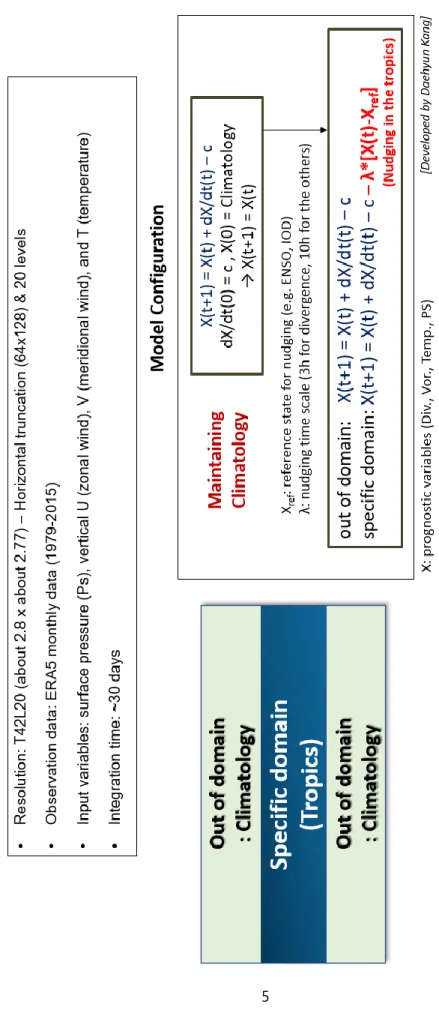
4 2.2 Model Experiments
194
To focus on dynamics from low to high latitude, the Geophysical Fluid Dynamics Laboratory 195
(GFDL; Hoskins et al. 2012) atmospheric model is used. This idealized model is the spectral dry 196
dynamical core of an atmospheric general circulation model from NOAA. The GFDL model has a 197
resolution T42 and 20 sigma coordinate levels. The model is initialized with the climatological 198
background of the ERA5 reanalysis for the austral spring from 1979 to 2015. To balance the model with 199
climatological state, the first time-step tendency is always subtracted at the next time-step and the 200
nudging forcing is added to the model equation at every time step. This additional forcing is obtained 201
by integrating the model forward one-time step with the initial condition. Until a tropical heating is 202
introduced as an initial perturbation, this additional forcing neutralizes the model’s initial tendency, 203
putting the model into a steady state. This procedure ensures that the model response in each time step 204
is due only to the initial perturbation. Also, the geography is used to help understanding the enhanced 205
drag over land (Li et al. 2014). On the three levels (σ=0.975,0.925,0.875) a differential damping scheme 206
is used whereby the winds are damped to oceans and land, respectively. This is used to damp thermal 207
anomalies for the basic state. A ∇4 hyper-diffusion, with a time-scale of 6h on the smallest resolved 208
horizontal scale, is applied to the vorticity, divergence and temperature. Vertical diffusion is also 209
applied to the perturbation vorticity, divergence and temperature fields (Hoskins et al. 2012).
210
As in Fig. 1, the first time-step tendency is specified as C and subtracted every time-step so that the 211
mean state is maintained and there is no error due to model bias. In the specific domain, a nudging term 212
is added here. To check the maintenance of the climatological background, the first 6 days repeat this 213
process without the forcing. After day 7, nudging in the tropics in a specific domain starts up integration 214
with λ which is a constant value that controls the nudging rate, X is the prognostic variable, and Xref is 215
a value that partially applies the climatology of reference state. Moreover, to identify the contribution 216
of each Ocean sector, the nudging domain is divided into four sectors, Tropics (30°N-30°S), Pacific 217
Ocean sector (30°N-30°S, 60°W-120°E), Indian Ocean sector (30°N-30°S, 30°-120°E), and Atlantic 218
Ocean sector (30°N-30°S, 120°-180°E). This study conducted several experiments by differing the 219
nudging domain, for example, with ENSO and IOD regression patterns applied in it.
220 221 222 223 224
5 225
Fig. 2. Schematics of GFDL dry dynamical core model
6
3. Results
226
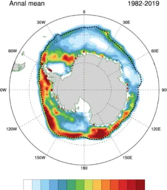
3.1 Climatological characteristics of Sea ice concentration 227
Antarctica divided into the East and the West Antarctica based on the transantarctic mountains. Fig. 1 228
indicates the annual mean variance of SIC. Compare to the East Antarctic, the West Antarctic has a large 229
interannual variability at the edge line of SIC climatology line. However, the variance of East Antarctic 230
SIC is smaller than west. Therefore, this study focuses on the variance of West Antarctica SIC. Antarctic 231
sea ice, as is well known, has a seasonal cycle for extent and concentration with minimum in February 232
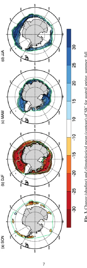
and maximum in October (Parkinson 2019). Fig. 2 displays the climatological-mean SIC (contour) and 233
the change of SIC (shading) for each season. Here, SIC-change was calculated by subtracting the value 234
of the preceding month. That is, Fig. 1 shows only the change in sea ice concentration for each season.
235
Since red shading represents a decrease in sea ice and blue shading represents an increase, (a) and (b) 236
are defined as the melting season and (c) and (d) as the growing season. Also, since the sea ice starts 237
decreasing at November, the SIC change is insignificant in (a). Characteristically, all other seasons have 238
shading inside the climatological-mean contour line, only the DJF outside. The SIC change in DJF has 239
a shape similar to the climatological-mean contour line of SON, which means that DJF is affected by 240
the increase of sea ice in SON. In (c), the smallest of Fig. 2, given that the SIC change between the 241
Weddell and some parts of the Ross Sea is close to zero, that part is considered a large ice shelf. Finally, 242
in (d), the SIC is growing from structure of (c).
243
Fig. 2. Annual mean variance (shading) and climatological mean (contour) of sea ice concentration 244
(SIC) anomalies during 1982-2019 245
7
246
Fig. 3. Change (shading) and climatological mean (contour) of SIC for austral spring, summer, fall, and winter from the left
8
3.2 Teleconnection between the tropics and southern high latitudes 247
This section addresses the remote influences of low latitude on the Antarctic.
248
249
Fig. 4. Regression of Sea Surface temperature (SST) and 500mb geopotential anomalies on Ocean Nino 250
Index (ONI) in austral winter, spring, and summer from the left. Black dot indicates the significant 251
regions at the 95% confidence level.
252
9
As mentioned in Section 1, ENSO is the most widely known phenomenon in the interannual time- 253
scale. When Z500 is regressed onto ENSO index (Fig. 4, contour), the jet stream is strongest in (a), and 254
it becomes smaller following the season. On the other hand, the El Nino pattern (Fig. 4, shading) in the 255
Pacific Ocean gets stronger. In turn, the most distinct remote patterns from low to high latitudes are 256
shown in (b), which is consistent with the results of previous studies (Jin and Kirtman 2010; Schneider 257
et al., 2012a). Besides, the austral spring season is also the peak season of IOD and the developing 258
season of ENSO. For this reason, this study focused on SON (September-October-November) among 259
the sea ice melting seasons.
260
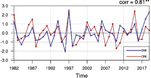
Fig. 5 shows the time series of the ENSO index (hereinafter, ONI) and the IOD index (hereinafter, 261
DMI) in SON. The correlation coefficient of the two indices is 0.61, which means that the fluctuations 262
of the two phenomena are considerably similar. That is, positive(negative) ENSO is related to 263
positive(negative) IOD. According to previous studies, since ENSO and IOD induce different Rossby 264
wave paths, when they occur simultaneously, Rossby waves propagate deeply to the Antarctic Peninsula, 265
whereas when only IOD occurs, they affect only the Ross Sea.
266
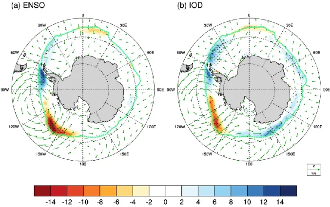
When the SIC and winds at 850mb are regressed onto each index (Fig. 6), a dipole pattern is observed 267
that increases sea ice in the Antarctic Peninsula and decreases sea ice in the Amundsen Sea. The little 268
difference is ENSO induces the SIC melting in the ABS, whereas IOD leads to wide melting in ABS 269
and the growth of sea ice in the Weddell Sea and East Antarctic. Also, the wind field in West Antarctica 270
is similar in (a) and (b), and in (a), there is no significant change in East Antarctica, whereas in (b), a 271
significant signal is observed. This means that ENSO is more related to sea ice in West Antarctica and 272
the sea ice pattern in East Antarctica is more related to IOD. Meanwhile, sea ice melting patterns appear 273
to be affected by the high-pressure atmospheric circulation over the ABS.
274
275
Fig. 5. The timeseries of ENSO index (red line) and IOD index (blue line). The correlation coefficient 276
between ENSO and IOD indices is 0.61 277
10 278
Fig. 6. Regression of SIC (shading) and 850mb winds (vector) anomalies on ENSO index (a) and IOD 279
index (b). Green line means climatological mean of SIC in austral spring. Black dot indicates the 280
significant regions at the 95% confidence level.
281 282 283
To understand the mechanisms for sea ice changes, the temperature advection is regressed onto each 284
index and analyzed (Fig. 7). Wind blowing from the Antarctic due to this atmospheric circulation pattern 285
causes cold advection, growing the sea ice near the Antarctic Peninsula. On the other hand, the wind 286
blowing from low latitudes causes warm advection, contributing to melting sea ice on the Amundsen 287
sea. That is, a thermodynamic mechanism impacts the sea ice of the West Antarctic during austral spring, 288
so the atmospheric circulation located in the West Antarctic (hereinafter, ABSH) has a great influence 289
on the sea ice dipole pattern. On the other hand, in (b), the cold advection is stronger than (a), especially 290
in the Indian Ocean and West Pacific Ocean sectors, accounting for sea ice increase in these regions 291
(Fig. 5b).
292 293
11 294
Fig. 7. Regression of temperature advection on ENSO index (a) and IOD index (b). Blue (red) vectors 295
indicate cold advection (warm advection).
296 297 298
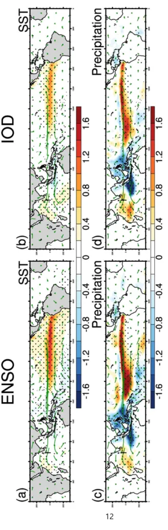
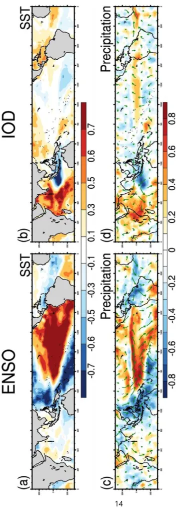
To find out where and how ENSO and IOD influence this circulation pattern, the convection location 299
in the tropics was first confirmed by the regression analysis of sea surface temperature and precipitation 300
(Fig. 8). As expected, the ENSO has an apparent SST pattern in the Pacific Ocean, and IOD shows a 301
distinct SST pattern in the Indian Ocean. However, since a high correlation coefficient between ENSO 302
and IOD, the overall patterns are almost identical. In other words, IOD regression displays a signal not 303
only Indian Ocean but also Pacific Ocean.
304 305 306
12
307
Fig. 8. Regression of SST (top panel), precipitation (bottom panel), and 850mb winds (vectors) on ONI (left) and DMI (right). Black dot indicates the significant regions at the 95% confidence level.
13
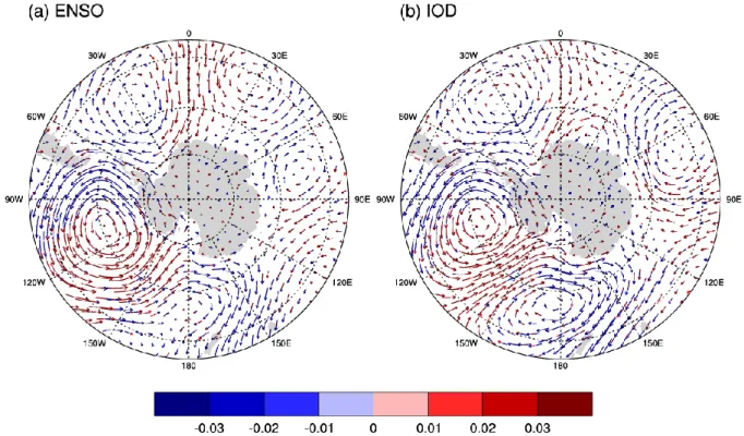
Fig. 9 displays the propagation pathway from low to high latitude, and 500mb geopotential height is 308
regressed onto ONI and DMI. The propagation pathway of ENSO seems to penetrate from South Pacific 309
judging from the low-pressure anomaly center at 150°W. Meanwhile, the propagation pathway of IOD 310
penetrates the south of Australia. Also, IOD is characterized by generating low-pressure signals at 60°- 311
90°E, inducing sea ice growing. The two phenomena seem to affect both ABSH and Antarctic dipole 312
pattern similarly.
313
314 315
316
Fig. 9. Regression of 500mb geopotential height (shading) and Rossby wave activity flux (WAF, vector) 317
on ONI (a) and DMI (b). Black dot indicates the significant regions at the 95% confidence level.
318 319 320 321
14
322
Fig. 10. Partial regression of SST (top panel) and precipitation (bottom panel) on the ONI (left) and DMI (right). Vector indicates winds at 850mb.
15
To isolate the individual impacts from ENSO and IOD, a partial regression analysis was additionally 323
conducted. When the ENSO and IOD indices are removed from each other, the regressed patterns onto 324
SST and precipitation (Fig. 10) show the responses mainly in the Pacific Ocean for ENSO and located 325
in the Indian Ocean for IOD respectively. So the two indices can be said to be well separated.
326 327 328
329
Fig. 11. Partial regression of 500mb geopotential height (shading) on ONI (a) and DMI (b) 330
331
Previous studies suggested that IOD alone does not affect sea ice in the eastern part of the Ross Sea.
332
However, Fig. 11b confirmed that pressure anomaly is transmitted to the coast of the ABS region and 333
near the Antarctic Peninsula. This means that IOD itself can cause sea ice variation near the Antarctic 334
Peninsula. Nonetheless, since this statistically eliminated the effect of ENSO on the IOD, it may have 335
resulted in an overall weakening of the response. Therefore, it is necessary to investigate the mechanical 336
mechanism through a model experiment.
337 338 339 340
16
3.3 GFDL model experiment
341 342
Using observation data, there is a hypothesis that ENSO and IOD influence the atmospheric circulation 343
and sea ice concentration patterns in West Antarctica, but how and which phenomena more affect to 344
West Antarctic has not been dynamically verified. Therefore, through the GFDL model experiment, 345
dynamic verification of the relationship between the Pacific, Indian Ocean, and West Antarctic 346
atmospheric circulation is performed. (Refer to Sector 2. for the explanation of basic model settings) 347
The climatological mean of SON is put in the background, and the regression pattern was put in the 348
nudging domain. Fig. 12 shows the regression pattern for SLP, 500mb winds, and air temperature at 349
500mb. In (a) displays a noticeable high-pressure pattern in the Indian Ocean, whereas the air 350
temperature of (c) is not clear. Similarly, air temperature in (d) also exhibits a weak pattern in the Indian 351
Ocean. Since each other’s influence was not excluded, the pattern related to ENSO has a signal not only 352
the Pacific Ocean but also the Indian Ocean. In the same manner, the pattern associated with IOD has 353
a sign in the Pacific Ocean too.
354 355
Fig. 12. Regression of SLP, winds (top panel), and air temperature at 500mb (bottom panel) on ONI (left) and DMI (right).
17
The first experiment generally nudges the ENSO regression pattern in the Pacific Ocean sector and 356
the IOD regression pattern in the Indian Ocean sector. In Fig. 13a and Fig. 13b, considering the low- 357
pressure anomaly center's location, the model results can catch observation results well. The top panel 358
shows different Rossby waves pathways, and the effect on ABSH and Antarctic dipole pattern (ADP) 359
was greater for ENSO than for IOD. Although IOD also minorly contributes to enhancing ABSH.
360
The second experiment nudges the ENSO pattern in the Indian Ocean sector and IOD pattern in the 361
Pacific sector by switching sectors (Fig. 13c and Fig. 13d). One peculiarity is that the impact of IOD is 362
greater in the Pacific than in the Indian Ocean. Thus, in order of influence, (a), (d), (b), and (c), it can 363
be seen that the overall influence on ABSH and ADP is stronger in the Pacific sector than in the Indian 364
Ocean sector. These results highlight the high correlation between ENSO and IOD.
365
To more accurately determine the influence of each of ENSO and IOD, model experiments were 366
conducted in the same manner using partial regression results. Fig. 14 shows the results of an 367
experiment that nudged ENSO and IOD partial regression patterns over the entire tropics (30°S-30°N).
368
Compared with Fig. 13, the overall strength was weakened, but the propagation pathway was almost 369
similar. ABSH and Antarctic dipole pattern induced by ENSO is also similar to the result of linear 370
regression. However, the partial regression for IOD significantly differs from observation. For example, 371
there is no ABSH related pattern in (b). Instead, the high-pressure shifted to onshore from the Ross Sea 372
to the Amundsen Sea. This result corresponds with the previous study (Nuncio and Yuan 2014).
373
However, these are also used as a statistical method such as partial regression, so there is a limit to fully 374
understanding.
375
Although the limitation of partial regression is that when removing the effects of ENSO from IOD, a 376
significant portion can be eliminated. Thus, ENSO and IOD can’t separate each other in reality. Fig. 15 377
shows the nudging results in Tropics domain (30°S-30°N) for ENSO (a) and IOD (b). Comparing with 378
previous model results, the effect induced by ENSO is not changed, but IOD is not. (b) is resembled 379
with Fig. 13 (d) and considerably different with Fig. 14 (b). This means that the IOD leading pattern is 380
more related to the Pacific Ocean sector than ENSO. Also, (a) and (b) are very similar in ABS, but 381
looking at the low-pressure center of the data line, those have different propagation pathways.
382 383 384
18 385
386 387
Fig. 13. Geopotential height (shading) and winds (vector) at 500mb anomalies at day 24 regarding ENSO and IOD regression pattern over Pacific Ocean (30°S-30°N ,60°W-120°E) and Indian Ocean (30°S-30°N, 30°-120°E) with the climatological mean as basic state during austral spring.
19 388
Fig. 14. Geopotential height (shading) and winds (vector) at 500mb anomalies at day 24 regarding 389
partial regression pattern of ENSO and IOD over Tropics (30°S-30°N) with the climatological mean as 390
basic state during austral spring 391
392
Fig. 15. As in Fig. 14 but for geopotential height (shading) and winds (vector) at 500mb anomalies 393
linearly regressed onto ENSO and IOD 394
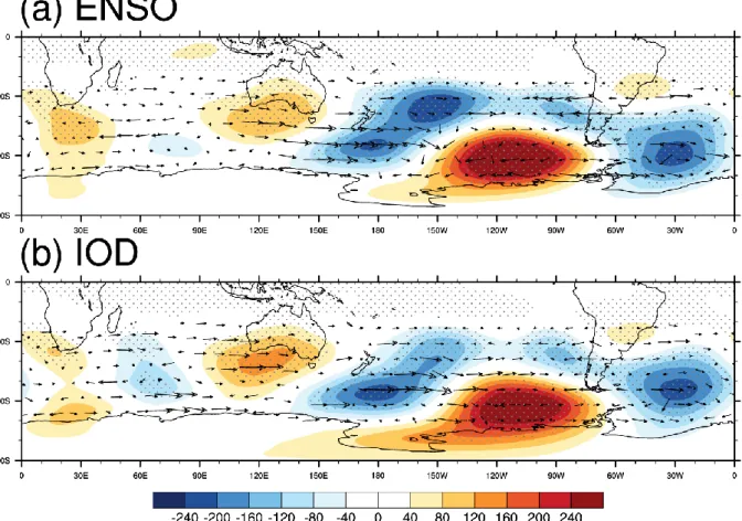
20 395
Fig. 16. Geopotential height (shading) and winds (vector) at 500mb anomalies at day 24 regarding 396
regression pattern of ENSO and IOD over Tropics (30°S-30°N) with the climatological mean as basic 397
state during austral spring 398
399 400
401
Fig. 17. As in Fig. 16 but for IOD over (b) Indian Ocean (30°S-30°N, 30°-120°E), (b) Pacific Ocean 402
(30°S-30°N ,60°W-120°E), (c) Atlantic Ocean (30°S-30°N, 120°-180°E) 403
21
To figure out which sector has the greatest influence among the tropical region, additional experiments 404
proceed, including the Atlantic Ocean sector. Fig. 16 shows the results by dividing ENSO effects into 405
the Pacific Ocean, Indian Ocean, and Atlantic Ocean sectors (see Section 2. for details). Both ENSO 406
and IOD contributed to form the ABSH pattern. Meanwhile, the external low-pressure pattern is mainly 407
formed by the Pacific Ocean sector. ENSO is most associated with the Pacific sector, high pressure in 408
ABS is associated with the Pacific and Indian Ocean sectors, and data lines and the Weddell Sea 409
cyclones appear to be affected by the Pacific and Atlantic sectors.
410
The experiment was conducted in the same way as in Fig. 17, but it’s the results of IOD. The pattern 411
of Fig. 14b seems to be more evenly affected by each sector than ENSO. For example, the low-pressure 412
anomaly in southeast Australia is largely influenced by the Indian Ocean, the high pressure in Antarctica 413
near the ABS is influenced by the Pacific Ocean, and ABSH seems to be offset by the influence of the 414
Atlantic Ocean. Alternatively, IOD in the Pacific sector (Fig. 17b) affects the interior of West Antarctica.
415
That is, GFDL model experiments simulate patterns similar to observations, and ABSH is more 416
affected by ENSO than IOD, and most of them originate from the Pacific Ocean. IOD has a weaker 417
effect than ENSO because the Rossby waves propagated from the Atlantic Ocean create a cyclone in 418
the Amundsen Sea and thus cancel out ABSH.
419
22
4. Summary and Discussion
420
This study examined the effects of ENSO and IOD on the sea ice of the West Antarctic in the austral 421
spring on the interannual time-scale. The correlation coefficient between the indices of ENSO and IOD 422
is about 0.61, and then synergistically affect the sea ice in Antarctica. Each phenomenon creates a dipole 423
pattern that thermodynamically reduces ABS sea ice and increases sea ice on the Antarctic Peninsula 424
through temperature advection caused by anticyclonic atmospheric circulation. According to the results 425
of regression analysis, the increase in sea ice in South Antarctica is related to IOD rather than ENSO.
426
To check the Rossby wave propagation pathway of each, 500mb geopotential height regressed onto 427
each index. Both ENSO and IOD induces high-pressure atmospheric circulation in the ABS, but at the 428
low-pressure anomaly center around the date line, the propagation pathway of IOD is located at a higher 429
latitude. On the other hand, ENSO propagates to the Antarctic through east Australia, and this result is 430
consistent with previous studies.
431
According to the GFDL model experiment results, the ENSO in the Pacific Sector has the most 432
influence on the West Antarctic atmospheric circulation, and the IOD has a weaker effect than that. The 433
reason why IOD has a weaker effect than ENSO is that the Rossby waves propagated from the Atlantic 434
Ocean create a cyclone in the Amundsen Sea, which offsets ABSH. Also, compared to ENSO, IOD 435
seemed to be influenced by domain. This is because, in the GFDL experiment, ENSO showed similar 436
results in which domain was nudged, but IOD showed different patterns according to domain settings.
437
When progress partial regression for IOD in the Tropics domain, as in previous studies, does not affect 438
the sea ice east of the Ross Sea but affects the interior of the Ross Sea, but in reality, ENSO and IOD 439
occur simultaneously. In other words, both ENSO and IOD contribute to the formation of ABSH, but 440
ENSO is stronger to the extent.
441
These results investigated how ENSO and IOD affect the atmospheric circulation and sea ice patterns 442
in West Antarctica, respectively. This will help predict the melting pattern of West Antarctic sea ice 443
according to the trends of ENSO and IOD. Since this study did not deal with the relationship between 444
IOD and the Atlantic Ocean and trend, further studies are needed to figure out the influence of the phase 445
of each phenomenon. Furthermore, there are few studies associated with the teleconnection from high 446
latitude to low latitude, so if it figures out, it will help to understand the southern hemisphere 447
atmospheric circulation cycle that affects Antarctic sea ice.
448 449
23
References
450
1. Bals-Elsholz, T. M., Atallah, E. H., Bosart, L. F., Wasula, T. A., Cempa, M. J., & Lupo, A. R.
451
(2001). The wintertime Southern Hemisphere split jet: Structure, variability, and evolution.
452
Journal of climate, 14(21), 4191-4215.
453
2. Baines, P. G., & Fraedrich, K. (1989). Topographic effects on the mean tropospheric flow 454
patterns around Antarctica. Journal of the Atmospheric Sciences, 46(22), 3401-3415.
455
3. Bromwich, D. H., Nicolas, J. P., Monaghan, A. J., Lazzara, M. A., Keller, L. M., Weidner, G.
456
A., & Wilson, A. B. (2013). Central West Antarctica among the most rapidly warming regions 457
on Earth. Nature Geoscience, 6(2), 139-145.
458
4. Board, O. S., & National Academies of Sciences, Engineering, and Medicine. (2017). Antarctic 459
Sea Ice Variability in the Southern Ocean-Climate System: Proceedings of a Workshop.
460
National Academies Press.
461
5. Chen, B., Smith, S. R., & Bromwich, D. H. (1996). Evolution of the tropospheric split jet over 462
the South Pacific Ocean during the 1986–89 ENSO cycle. Monthly weather review, 124(8), 463
1711-1731.
464
6. Clem, K. R., & Renwick, J. A. (2015). Austral spring Southern Hemisphere circulation and 465
temperature changes and links to the SPCZ. Journal of Climate, 28(18), 7371-7384.
466
7. Eayrs, C., Holland, D., Francis, D., Wagner, T., Kumar, R., & Li, X. (2019). Understanding the 467
Seasonal Cycle of Antarctic Sea Ice Extent in the Context of Longer‐Term Variability. Reviews 468
of Geophysics, 57(3), 1037-1064.
469
8. Gong, T., Feldstein, S., & Lee, S. (2017). The role of downward infrared radiation in the recent 470
Arctic winter warming trend. Journal of Climate, 30(13), 4937-4949.
471
9. Hannachi, A., & Dommenget, D. (2009). Is the Indian Ocean SST variability a homogeneous 472
diffusion process?. Climate dynamics, 33(4), 535-547.
473
10. Holland, P. R., & Kwok, R. (2012). Wind-driven trends in Antarctic sea-ice drift. Nature 474
Geoscience, 5(12), 872-875.
475
11. Hoskins, B., Fonseca, R., Blackburn, M., & Jung, T. (2012). Relaxing the tropics to an 476
‘observed’state: Analysis using a simple baroclinic model. Quarterly Journal of the Royal 477
Meteorological Society, 138(667), 1618-1626.
478
12. Jin, D., & Kirtman, B. P. (2010). How the annual cycle affects the extratropical response to 479
ENSO. Journal of Geophysical Research: Atmospheres, 115(D6).
480
13. Karoly, D. J. (1989). Southern hemisphere circulation features associated with El Niño- 481
Southern Oscillation events. Journal of Climate, 2(11), 1239-1252.
482
14. Labe, Z., Peings, Y., & Magnusdottir, G. (2018). Contributions of ice thickness to the 483
atmospheric response from projected Arctic sea ice loss. Geophysical Research Letters, 45(11), 484
5635-5642.
485
15. Lee, H. J., & Seo, K. H. (2019). Impact of the Madden-Julian oscillation on Antarctic sea ice 486
and its dynamical mechanism. Scientific reports, 9(1), 1-10.
487
24
16. Liu, J., Yuan, X., Rind, D., & Martinson, D. G. (2002). Mechanism study of the ENSO and 488
southern high latitude climate teleconnections. Geophysical Research Letters, 29(14), 24-1.
489
17. Li, X., Holland, D. M., Gerber, E. P., & Yoo, C. (2014). Impacts of the north and tropical 490
Atlantic Ocean on the Antarctic Peninsula and sea ice. Nature, 505(7484), 538-542.
491
18. Li, X., Gerber, E. P., Holland, D. M., & Yoo, C. (2015). A Rossby wave bridge from the tropical 492
Atlantic to West Antarctica. Journal of Climate, 28(6), 2256-2273.
493
19. Massom, R. A., Eicken, H., Hass, C., Jeffries, M. O., Drinkwater, M. R., Sturm, M., ... & Morris, 494
K. (2001). Snow on Antarctic sea ice. Reviews of Geophysics, 39(3), 413-445.
495
20. Massom, R. A., & Stammerjohn, S. E. (2010). Antarctic sea ice change and variability–physical 496
and ecological implications. Polar Science, 4(2), 149-186.
497
21. Miles, B. W., Stokes, C. R., & Jamieson, S. S. (2016). Pan–ice-sheet glacier terminus change 498
in East Antarctica reveals sensitivity of Wilkes Land to sea-ice changes. Science advances, 2(5), 499
e1501350.
500
22. Mo, K. C., & Higgins, R. W. (1998). The Pacific–South American modes and tropical 501
convection during the Southern Hemisphere winter. Monthly Weather Review, 126(6), 1581- 502
1596.
503
23. Nuncio, M., & Yuan, X. (2015). The influence of the Indian Ocean dipole on Antarctic sea 504
ice. Journal of Climate, 28(7), 2682-2690.
505
24. Parkinson, C. L. (2019). A 40-y record reveals gradual Antarctic sea ice increases followed by 506
decreases at rates far exceeding the rates seen in the Arctic. Proceedings of the National 507
Academy of Sciences, 116(29), 14414-14423.
508
25. Reynolds, R. W., Smith, T. M., Liu, C., Chelton, D. B., Casey, K. S., & Schlax, M. G. (2007).
509
Daily high-resolution-blended analyses for sea surface temperature. Journal of Climate, 20(22), 510
5473-5496.
511
26. Simmonds, I., Keay, K., & Lim, E. P. (2003). Synoptic activity in the seas around 512
Antarctica. Monthly Weather Review, 131(2), 272-288.
513
27. Shepherd, A., Fricker, H. A., & Farrell, S. L. (2018). Trends and connections across the 514
Antarctic cryosphere. Nature, 558(7709), 223-232.
515
28. Schneider, D. P., Deser, C., & Okumura, Y. (2012). An assessment and interpretation of the 516
observed warming of West Antarctica in the austral spring. Climate Dynamics, 38(1-2), 323- 517
347.
518
29. Turner, J., Phillips, T., Marshall, G. J., Hosking, J. S., Pope, J. O., Bracegirdle, T. J., & Deb, P.
519
(2017). Unprecedented springtime retreat of Antarctic sea ice in 2016. Geophysical Research 520
Letters, 44(13), 6868-6875.
521
30. Wu, X., Budd, W. F., Lytle, V. I., & Massom, R. A. (1999). The effect of snow on Antarctic sea 522
ice simulations in a coupled atmosphere-sea ice model. Climate Dynamics, 15(2), 127-143.
523
31. Yoon, S. T., Lee, W. S., Stevens, C., Jendersie, S., Nam, S., Yun, S., ... & Lee, J. (2020).
524
Variability in high-salinity shelf water production in the Terra Nova Bay polynya, Antarctica.
525
25
32. Yu, J. Y., Paek, H., Saltzman, E. S., & Lee, T. (2015). The early 1990s change in ENSO–PSA–
526
SAM relationships and its impact on Southern Hemisphere climate. Journal of Climate, 28(23), 527
9393-9408.
528
33. Yuan, X. (2004). ENSO-related impacts on Antarctic sea ice: a synthesis of phenomenon and 529
mechanisms. Antarctic Science, 16(4), 415-425.
530
34. Yuan, X., Kaplan, M. R., & Cane, M. A. (2018). The interconnected global climate system—
531
A review of tropical–polar teleconnections. Journal of Climate, 31(15), 5765-5792.
532
35. Zhang, J. (2007). Increasing Antarctic sea ice under warming atmospheric and oceanic 533
conditions. Journal of Climate, 20(11), 2515-2529.
534