Deadbeat-Based Model Predictive Voltage Control for a Sensorless Five-Phase Induction Motor Drive

(1)

Research Article

Deadbeat-Based Model Predictive Voltage Control for a Sensorless Five-Phase Induction Motor Drive

Mahmoud A. Mossa ,

¹

Nguyen Vu Quynh ,

²

Hamdi Echeikh ,

³

and Ton Duc Do

⁴

1Electrical Engineering Department, Faculty of Engineering, Minia University, Minia 61111, Egypt

2Electrical and Electronics Department, Lac Hong University, Dong Nai, Vietnam

3Department of Electrical Engineering, National Engineering School of Monastir, P.O. Box 5035, Monastir, Tunisia

4Department of Robotics and Mechatronics, School of Engineering and Digital Sciences (SEDS), Nazarbayev University, Nur-Sultan Z05H0P9, Kazakhstan

Correspondence should be addressed to Mahmoud A. Mossa; mahmoud_a_mossa@mu.edu.eg and Nguyen Vu Quynh;

vuquynh@lhu.edu.vn

Received 16 April 2020; Accepted 11 June 2020; Published 15 July 2020

Academic Editor: Salvatore Strano

Copyright © 2020 Mahmoud A. Mossa et al. This is an open access article distributed under the Creative Commons Attribution License, which permits unrestricted use, distribution, and reproduction in any medium, provided the original work is properly cited.

This paper introduces a direct model predictive voltage control (DMP VC) for a sensorless five-phase induction motor drive. The operation of the proposed sensorless DMP VC is based on the direct control of the applied stator voltages instead of controlling the torque and flux as in model predictive direct torque control (MP DTC). Thus, the simplicity of the control system is enhanced, which saves the computational time and reduces the commutation losses as well. The methodology based on which the proposed sensorless DMP VC performs its operation depends on minimizing a cost function that calculates the error between the reference and actual values of the direct and quadrature (d-q) axes components of stator voltages. The reference values ofd-qcomponents of stator voltages are obtained through incorporating the deadbeat control within the proposed model predictive system. A robust back-stepping observer is proposed for estimating the speed, stator currents, rotor flux, and rotor resistance. The validity of the proposed sensorless DMP VC is confirmed through performing detailed and extensive comparisons between the proposed DMP VC and MP DTC approach. The obtained results state that the drive is exhibiting better performance under the proposed DMP VC with less ripples content and reduced computational burden. Moreover, the proposed back-stepping observer has confirmed its effectiveness in estimating the speed and other variables for a wide range of speed operation.

1. Introduction

Recently, the multiphase machine drives have been given great concern due to their various advantages compared with the three-phase AC machine drives [1–3]. These advantages can be addressed in the form of high robustness, smooth torque proﬁle, reduced ripples content in the controlled variables, reduced current rating for each phase of the stator, and enhanced fault-ride through capability [4–6].

All of these merits have motivated the industrial commu- nities to use the multiphase machines in high-power applications such as aircraft and naval propulsion and electric traction systems, as well as aerospace applications [7–9].

One of the most familiar types of multiphase machines is the five-phase induction motor (FPIM) [10–12]. Many control topologies have been presented for controlling the operation of the FPIM drives so that an optimal performance can be obtained from the drive in terms of low ripple contents, high efficiency, and ease of practical imple- mentation. The direct torque control (DTC) and field oriented control (FOC) are considered as the most used control topologies for the majority of electric machine drives [13–16]. Both techniques have contributed effectively to improving the dynamic performance of the FPIM drive, but on the other hand they have suffered from some problems.

For example, for the FOC approach, the system complexity

Volume 2020, Article ID 4164526, 30 pages https://doi.org/10.1155/2020/4164526

(2)

is obvious due to the utilization of multiple proportional- integral (PI) controllers, which require precise tuning of its coeﬃcients. This is in addition to the time delay, which is added to the system response due to the use of PI controllers [13, 14]. On the other hand, the DTC control approach has managed to reduce the system complexity and achieve fast dynamic response as well. However, it has suﬀered from the remarkable ripples content in the controlled variables [15, 16].

To overcome the shortages of the DTC and FOC ap- proaches, the model predictive control (MPC) principle has been presented for the FPIM drive in diﬀerent forms. Some of these forms have depended on controlling the torque and ﬂux and were entitled as model predictive direct torque control (MP DTC) [12, 17]. The MP DTC approach has succeeded in reducing the system complexity and reducing the ripples compared with the classic DTC look-up table based approach, but the ripples have not been totally suppressed.

However, the MP DTC has suﬀered from the high computational burden, which cannot be realized by all microprocessors. The main factor that manages the computation time in the model predictive control in general is the form and parts of the used cost function. For example, for the MP DTC, the cost function is consisting of two parts:

one for the torque regulation and the other for the ﬂux management. This function type requires the utilization of a weighting factor to weigh the importance of each term with respect to the other. The calculation of optimal weighting factor is a time-consuming process, which results in adding extra execution time and increasing the commutation losses.

This is in addition to the fact that both terms (torque and ﬂux) need to be estimated, which again lengthens the computational time for each cycle.

As a solution for these issues, the current paper proposes a direct model predictive voltage control (DMP VC) approach for a sensorless FPIM drive. The operation of the proposed approach is based upon utilizing a cost function form, which consists of two similar terms to avoid using a weighting factor. The two similar terms of the cost function are the errors between the reference values of direct- quadrature (d-q) axes components of stator voltage and their correspondent actual values. Through checking the cost function conﬁguration as will be illustrated later, it can be realized that the cost function’s variables (the voltages applied to the motor terminals) can be directly accessed without performing any estimation. This procedure has resulted in reducing the calculation time of the cost function, which reduces the commutation time as well as switching power losses. Moreover, the control is now dealing directly with the fastest variable to be applied to the PFIM (which is here the stator voltage), and this results in enhancing the system dynamic response.

To increase the robustness of the FPIM drive, several sensorless schemes have been proposed for estimating the rotor speed and rotor ﬂux. Some of them have depended on utilizing the model reference adaptive system (MRAS) observer [18–20]. The main deﬁciency of the MRAS observer is the sensitivity to parameters variation, especially at low

speed operation. Other sensorless schemes have utilized the sliding mode observer [21, 22]. The precision of the speed estimation using the sliding mode observers has been negatively aﬀected by the noise characteristics. Moreover, in order to solve the chattering problem, higher-order sliding modes have been utilized, which resulted in increasing the system’s complexity. Another senseless procedure has implemented the extended Kalman ﬁlter for estimating the speed [23]. The main issue related to this scheme is the dependency of the observer’s model on the parameters, which can result in deteriorating the estimation due to the parameters variation under certain operating conditions.

Another scheme has depended on estimating the rotor position through tracking the saliency position [24]. This method has suﬀered from the increased computational capacity of the system due to the system complexity.

As an attempt to achieve robust and precise speed estimation without adding extra computational burden on the controller, a new back-stepping speed observer is presented in this paper. The proposed back-stepping observer not only estimates the speed but also estimates the stator current, the rotor flux, and rotor resistance. Checking the observer’s stability has been presented to confirm its effectiveness in estimating the speed precisely for a wide range of operations under varying the rotor resistance. It is worth mentioning that the back-stepping principle has been introduced for different AC machine drives as a control system [25, 26], but it has been rarely utilized as a speed observer.

The back-stepping approach is a recursive procedure, the operation of which is based on the Lyapunov theory. This strategy is widely used for designing the control laws for uncertain systems. To our knowledge, majority of the methods that have been used for observing the states of the induction machine depending on the back-stepping principle and introduced in the literature have been mainly utilized for estimating the resistive and inductive parameters of the machine in the presence of mechanical speed sensor.

However, the difficulties are coming out when eliminating the speed sensor because of the unobservability of the motor, especially at very low speed. It is shown that the proposed method in [27] must be modified to take into account this nonlinear dynamic coupling by introducing other damping terms into each control input. The second contribution that the paper presents is to apply the back-stepping observer to the systems that have high degree of coupling between the electromagnetic and mechanical variables. In this form, the nonlinearities entering each subsystem are allowed to de- pend on the output associated with the subsystem and the states of the upper subsystem, including the unmeasured ones. The proposed observer algorithm is applied to the five- phase induction motor. The proposed observer only takes the stator voltages and currents as inputs and provides the speed, the rotor flux, the stator current, and rotor resistances as estimated outputs.

The paper is organized as follows; it starts with introducing the mathematical model of the ﬁve-phase IM (FPIM) drive. Then, in Section 3, the proposed DMP VC approach is described and analyzed in detail. After that, in Section 4, the proposed back-stepping observer is presented and

(3)

explained. In Section 5, the complete system conﬁguration is presented. In Section 6, the test results are introduced and discussed. The test results are presented in the form of comprehensive comparisons between the proposed DMP VC and MP DTC approach. Finally, Section 7 introduces the conclusion and the outcomes of the paper.

The contributions of the paper can be addressed through the following items:

(i) The proposed DMP VC approach has not been tested before with the FPIM drive.

(ii) The derivation and analysis of the proposed DMP VC are performed through a detailed mathematical veriﬁcation so that the base principle can be easily understood.

(iii) The proposed back-stepping observer has been presented and analyzed in detail so that the operation principles of the observer can be easily veriﬁed.

(iv) The robustness of the proposed back-stepping observer has been veriﬁed under the parameters variation for a wide range of speed operation.

(v) A detailed comparison between the proposed DMP VC and MP DTC for the FPIM drive is carried out in terms of the total harmonic distortion (THD) for the current signals and in terms of the average error values. Moreover, a comparison has been carried out in terms of switching frequencies and number of commutations and ﬁnally in terms of the computational time and switching losses.

2. Mathematical Model of FPIM

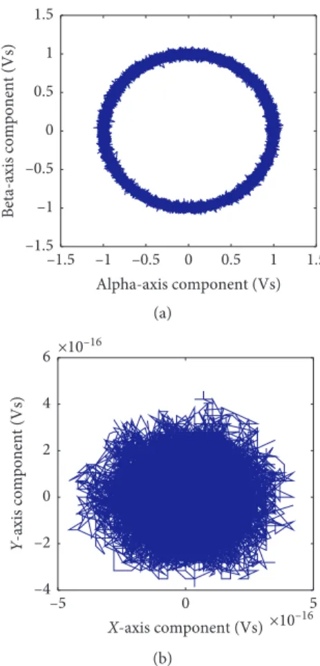
Several studies have presented and formulated the mathematical model of FPIM according to specific assumptions [28, 29]. The model can be represented in different reference frames, such as the rotating synchronous reference frame, which gives the (d-q-x-y) axes configuration, while representing the model in the stationary reference frame gives the (α-β-z₁-z₂) axes configuration.

When representing the FPIM model in the synchronous reference frame, the d-q components will be responsible for managing the ﬂux and torque, respectively.

Meanwhile, the x-y components will be responsible for developing the losses.

Under rotor ﬁeld oriented control (RFOC), the following discretized relationships are obtained at instant kTs as follows:

ψ^rf_dr,k�􏼌􏼌􏼌􏼌􏼌ψ^rf_r,k􏼌􏼌􏼌􏼌􏼌, ψ^rf_qr,k �0.0,

(1)

where Ts is the sampling time;ψ^rf_dr,k and ψ^rf_qr,k refer to the direct and quadrature axes components of stator flux defined in the synchronous rotating frame. Moreover, the superscript “rf” is used to state that the variables are defined in a reference frame, which rotates synchronously with the rotor flux.

Utilizing (1) and via adopting the principles of RFOC, the equations that describe the electric dynamics of the FPIM can be represented in the (d-q-x-y) reference frame by

dψ^rf_dr,k dt �dψ^rf_r,k

dt �L_m τr

i^rf_ds,k− ψ^rf_dr,k τr

, (2)

dψ^rf_qr,k

dt �0.0�L_m

τ_ri^rf_qs,k− ω_sl,kψ^rf_dr,k, (3) di^rf_ds,k

dt �c₁i^rf_ds,k+ω_me,ki^rf_qs,k+c₂ψ^rf_dr,k+ 1

L_tu^rf_ds,k, (4) di^rf_qs,k

dt �c₁i^rf_qs,k− ω_me,ki^rf_ds,k+c₂ψ^rf_dr,k+ 1

L_tu^rf_qs,k, (5) di^rf_xs,k

dt �−R_s L_lsi^rf_xs,k+ 1

L_lsu^rf_xs,k, (6) di^rf_ys,k

dt �−R_s L_lsi^rf_ys,k+ 1

L_lsu^rf_ys,k, (7) dωme,k

dt �c₃ψ^rf_dr,ki^rf_qs,k− p

JT_l,k, (8)

where the subscripts s andr refer to the stator and rotor variables, respectively, and

c₁�L²_mR_r+L²_rR_s L_tL²_r , c₂�L_mR_r

L_tL_r, c₃�p²L_m

JL_r , ω_sl�ω_ψ_r− ω_me,

(9)

whereω_ψ_ris the angular frequency of the rotor ﬂux,ω_meis the mechanical angular frequency, andω_slis the slip angular frequency. The parametersR_sandR_rrefer to the stator and rotor resistances, respectively. The inductances L_s, L_r, L_m, and L_ls refer to the stator, rotor, magnetizing, and stator leakage inductances, respectively. The inductance L_t�σL_s refers to the stator transient inductance, while the constant σ �1− (L²_m/L_sL_r) refers to the total leakage factor. The parameterspandJrefer to the pole pairs and the moment of inertia, respectively. Finally, τ_r�L_r/R_r refers to the rotor time constant.

Via utilizing the relationships (2) to (8), the equivalent circuit of the FPIM can be represented as shown in Figure 1.

In this ﬁgure, it can be noticed that the model is consisting of decoupled d-q axes equivalent circuits similar to those of three-phase IM, decoupledx-yaxes equivalent circuits, and decoupled x-y axes equivalent circuits for the rotor. The latter can be simply represented by resistive-inductive circuits.

(4)

3. The Proposed DMP VC Approach

The principle based upon which the proposed DMP VC approach is formulated states that the motor’s ﬂux and torque can be directly controlled via controlling the direct and quadrature (d-q) axes components of applied stator voltage (u^rf_ds,k, u^rf_qs,k), respectively. This argument can be veriﬁed mathematically as follows.

Under RFOC, the total rotor ﬂux is aligned with thed- axis of the rotating reference frame, and the following relationships are obtained:

ψ^rf_r,k�L_ri^rf_r,k+L_mi^rf_s,k�L_mi^rf_mr,k, (10) wherei^rf_mr,kis the rotor magnetizing current andi^rf_s,kandi^rf_r,k are the stator and rotor current vectors, respectively.

The relationship between the stator, rotor, and magnetizing currents can be represented by

i^rf_mr,k �ψ^rf_r,k L_m � L_r

L_mi^rf_r,k+i^rf_s,k. (11) Under the RFOC, the reference frame rotates with an angular speed deﬁned by

ω_ψ_r,k�ω_me,k+ i^rf_qs,k

􏽺√􏽽􏽼√􏽻^ω^sl,k

τri^rf_mr,k

. (12)

The space vector representation under the application of RFOC is illustrated in Figure 2, through which it is observed that the total rotor flux is fixed with thed-axis of the rotating frame and rotates with an angular frequency of ω_ψ_r,k. The angleδ_krefers to the load angle (torque angle) between the rotor flux and stator current vectors. The stator current vector rotates with an angular frequency of ωs,k�d/dt(δk+θψ_r,k).

The voltage balance in the FPIM circuit can be expressed in an alternative form by the following relationships:

u^rf_s,k �R_si^rf_s,k+dψ^rf_s,k

dt +jωψ_r,kψ^rf_s,k, (13)

u^rf_r,k�0�R_ri^rf_r,k+dψ^rf_r,k

dt +j􏼐ω_ψ_r,k− ω_me,k􏼑

􏽺√√√√√􏽽􏽼√√√√√􏽻^ω^sl,k

ψ^rf_r,k. (14) By substituting (11) and (12) into (13) and (14), and after mathematical derivations, this results in

u^rf_ds,k�R_si^rf_ds,k+(1− σ)L_sdi^rf_mr,k

dt +σL_s di^rf_ds,k

dt − i^rf_qs,kω_ψ_r,k

􏼠 􏼡,

(15)

u^rf_qs,k �R_si^rf_qs,k+(1− σ)L_si^rf_mr,kω_ψ_r,k+σL_s di^rf_qs,k

dt +i^rf_ds,kω_ψ_r,k

⎛⎝ ⎞⎠,

(16)

+ –

– +

R_r L_lr R_s L_ls – +

ψ_qsrf

ω_ψ_r ω_slψ^rf_qr

i_ds i_dr^rf

urf_dr

urf_ds L_m

rf

(a)

R_r L_lr R_s L_ls

ψrf_ds

ω_ψ_r ωslψdr^rf i_qrrf

urf_qr

i_qsrf

– +

L_m

+ - – +

(b) R_s L_ls

R_s L_ls

urf_xs u_ys^rf

– –

+ +

i_xs^rf i_ys^rf

(c)

R_r L_lr R_r L_lr

i_xrrf iyr^rf

(d)

Figure1: (d-q-x-y) axes equivalent circuit model of FPIM deﬁned in synchronous reference frame. (a)d-axis equivalent circuit, (b)q-axis equivalent circuit, (c)x-yaxes equivalent circuits for stator side, and (d)x-yaxes equivalent circuits for rotor side.

Stator axis Rotor ﬂux axis

i_αs i_qs

θ_ψ^–_r

ω_ψ^–_r ω_s

δ i–

s

i_βs

i_ds = (ψ_r/L_m) = i_mr

Figure2: Vector diagram for steady-state operation of IM under RFOC.

(5)

τ_rdi^rf_mr,k

dt +i^rf_mr,k �i^rf_ds,k, (17) J

p dω_me,k

dt �1􏽼√√√√√√􏽻􏽺√√√√√√􏽽.5p(1− σ)L_s

∇

i^rf_mr,ki^rf_qs,k

􏽺√√√√√√√√√􏽽􏽼√√√√√√√√√􏽻^T^e,k

− T_l,k. (18) Using (17) and its derivative, by substituting into (15), this results in

u^rf_ds,k�σL_sτ_rd²i^rf_mr,k

dt² + R_sτ_r+L_s􏼁di^rf_mr,k dt +R_si^rf_mr,k− σL_si^rf_qs,kωψ_r,k.

(19)

By taking the Laplace transform of (19), this results in u^rf_ds,k(s) �σL_sτ_r􏼒s²i^rf_mr,k(s)􏼓+ R_sτ_r+L_s􏼁si^rf_mr,k(s)

+R_si^rf_mr,k(s) − σL_sL􏼐i^rf_qs,kω_ψ_r,k􏼑,

(20)

where L denotes Laplace transform. Then the value of i^rf_mr,k(s)can be derived from (20) by

i^rf_mr,k(s) � 1/R_s􏼁u^rf_ds,k(s) +στ_sL􏼐i^rf_qs,kω_ψ_r,k􏼑

στ_sτ_rs²+ τ_s+τ_r􏼁s+1 , (21) where τ_s is the stator time constant that is equal to τ_s�L_s/R_s.

The characteristic polynomial equation of the transfer function given by (21) has always real eigenvalues, which can be derived as follows:

στ_sτ_rs²+ τ_s+τ_r􏼁s+1�0.0,

s_1,2�− τ_s+τ_r􏼁 2στ_sτ_r ±

��

τ_s+τ_r􏼁²− 4στ_sτ_r

􏽱

2στ_sτ_r . (22) To get real eigenvalues, the quantity under root square

��

(τ_s+τ_r)²− 4στ_sτ_r

􏽱

must be larger than 0.0; thus, z�τ²_s+τ²_r+2τ_sτ_r− 4στ_sτ_r>0.0, (23) and thus (21) can be rewritten by

i^rf_mr,k(s) � 1/R_su^rf_ds,k(s) +στ_sL􏼐i^rf_qs,kω_ψ_r,k􏼑 2στ_sτ_r/ τ_s+τ_r− �

√z

􏼁􏼁s+1􏼁+ 2στ_sτ_r/τ_s+τ_r+ �

√z

􏼁s+1􏼁. (24)

From (24), it can be realized that the termL(i_qsω_ψ_r)can be recognized as a disturbance on which the control system has to be robust.

Now, from (10), (11), and (24), the transfer function that relates to the rotor ﬂux and the input d-axis stator voltage component can be expressed by

ψ^rf_r,k(s) � L_m/R_s􏼁u^rf_ds,k(s) 2στ_sτ_r/ τ_s+τ_r− �

√z

􏼁􏼁s+1􏼁+ 2στ_sτ_r/τ_s+τ_r+ �

√z

􏼁s+1􏼁

+ σL_mτ_sL􏼐i^rf_qs,kω_ψ_r,k􏼑 2στ_sτ_r/ τ_s+τ_r− �

√z

􏼁􏼁s+1􏼁+ 2στ_sτ_r/ τ_s+τ_r+ �

√z

􏼁s+1􏼁.

(25)

Assuming that, under steady-state operation, the current i^rf_mr,k is constant, from (16), the Laplace transform ofi^rf_qs,k(s) can be obtained and expressed by

i^rf_qs,k(s) �

1/R_s u^rf_qs,k

􏽺√􏽽􏽼√􏽻

−L_sL􏼐i^rf_qs,kω_ψ_r,k􏼑

􏼢 􏼣

στ_ss+1 . (26) From (25) and (26), the argument that states that the ﬂux and torque of the FPIM can be regulated using the d-q components of stator voltage is veriﬁed and approved. Then, via substitution from (12) and (18) into (26), the mathematical model of FPIM can be obtained in the functional diagrams as shown in Figures 3 and 4.

After approving the hypothesis of controlling the torque and ﬂux directly through controlling thed-qcomponents of the applied stator voltage, the cost function to be utilized by the proposed DMP VC can be formulated by

C^j_k�􏼌􏼌􏼌􏼌􏼌u_ds,k^∗ − u^rf_ds,k􏼌􏼌􏼌􏼌􏼌^j+􏼌􏼌􏼌􏼌􏼌u_qs,k^∗ − u^rf_qs,k􏼌􏼌􏼌􏼌􏼌^j+􏼌􏼌􏼌􏼌􏼌0.0− u^rf_xs,k􏼌􏼌􏼌􏼌􏼌^j+􏼌􏼌􏼌􏼌􏼌0.0− u^rf_ys,k􏼌􏼌􏼌􏼌􏼌^j, (27) where jdenotes the voltage index.

By checking the terms of the cost function (27), it can be realized that the terms are of the same type and thus there is no need to utilize a weighting factor, which saves the computation time. Moreover, it can be noticed that the controlled variables (the stator voltage componentsu^rf_ds,k,u^rf_qs,k,u^rf_xs,k, and u^rf_ys,k) can be directly obtained via three diﬀerent procedures;

the ﬁrst choice is obtained via direct measurements using ﬁlters, but this solution is not preferred due to the delay in the system response. The second way to get the voltage components is through calculating the voltages with the help of pulse width modulation (PWM) using the switching states, but this method results in varying and high-switching frequencies, which increases the switching losses. The third

(6)

method is to adopt the ﬁnite control set (FCS) principle and calculate the voltages from the switching states (Sa,Sb,Sc,Sd, andSe) of the inverter, and this method is adopted here due to

its simplicity and reduced computational burden. The calculation of the voltages using the switching states is illustrated by the following formulations:

u_as,k�U_dc

5 4S_a− S_b− S_c− S_d− S_e􏼁, u_bs,k�U_dc

5 4S_b− S_a− S_c− S_d− S_e􏼁, u_cs,k�U_dc

5 4S_c− S_a− S_b− S_d− S_e􏼁, u_ds,k�U_dc

5 4S_d− S_a− S_b− S_c− S_e􏼁, u_es,k�U_dc

5 4S_e− S_a− S_b− S_c− S_d􏼁, u^s_αs,k�

�2

5

􏽲

u_as,k+cos 2π

􏼒5􏼓u_bs,k+cos 4π

􏼒5􏼓u_cs,k+cos 4π

􏼒5􏼓u_ds,k+cos 2π

􏼒5􏼓u_es,k

􏼒 􏼓,

u^s_βs,k�

� 2 5

􏽲

sin 2π

􏼒5􏼓u_bs,k+sin 4π

􏼒5􏼓u_cs,k− sin 4π

􏼒5􏼓u_ds,k− sin 2π

􏼒5􏼓u_es,k

􏼒 􏼓,

u^s_xs,k�

�2

5

􏽲

u_as,k+cos 4π

􏼒5􏼓u_bs,k+cos 8π

􏼒5􏼓u_cs,k+cos 8π

􏼒5􏼓u_ds,k+cos 4π

􏼒5􏼓u_es,k

􏼒 􏼓,

u^s_ys,k�

�2

5

􏽲

sin 4π

􏼒5􏼓u_bs,k+sin 8π

􏼒5􏼓u_cs,k− sin 8π

􏼒5􏼓u_ds,k− sin 4π

􏼒5􏼓u_es,k

􏼒 􏼓,

(28)

+– στ_ss + 1

(1/R_s)

+–

J

p ω_me

T_l

Te

u_qs i_qs

++

ω_slip L_si_mr ω_ψ–_r

∇i_mr

Figure3: Control ofi_qs (torque regulation).

(L_m/R_s)

σLmτs

++

x

ψ_r u_ds

ω_ψ_r imr

τ_r + τ_s – 2στrτss

 + 1 τ_r + τ_s + 2στrτss

 + 1

τ_r + τ_s – 2στ_rτ_ss

 + 1 τ_r + τ_s + 2στ_rτ_ss

 + 1

Figure4: Control ofψ_r(ﬂux regulation).

(7)

where the superscript s refers to the quantities deﬁned in stationary frame. Then the feedback d-q-x-y stator voltage components deﬁned in the synchronous reference frame rf can be calculated by

u^rf_ds,k�u^s_αs,kcosθ_ψ_r,k+u^s_βs,ksinθ_ψ_r,k, u^rf_qs,k� −u^s_αs,ksinθ_ψ_r,k+u^s_βs,kcosθ_ψ_r,k, u^rf_xs,k�u^s_xs,kcosθψ_r,k+u^s_ys,ksinθψ_r,k, u^rf_ys,k� −u^s_xs,ksinθ_ψ_r,k+u^s_ys,kcosθ_ψ_r,k.

(29)

The reference values ofu_xs,k^∗ andu_ys,k^∗ are set to zero to minimize the power losses. The remaining parts of the cost function (27) are the reference values of stator voltage components u_ds,k^∗ and u_qs,k^∗ , which are derived through adopting the deadbeat control principle within the predictive voltage controller. This can be described as follows.

The deadbeat control has the ability to perform a simple and direct treatment of the controlled variables (torque, ﬂux, and current), as it enables the computation of the desired input signal (reference values) ensuring that the actual signals will track deﬁnitely the reference signals for each control cycle when applied to a discretized system. For this reason, the deadbeat control is utilized here to generate the references of the d-qcomponents of stator voltage vectors, which are then utilized by the cost function besides the actual d-qcomponents of stator voltage vectors (u_ds,k^∗ and u_qs,k^∗ ). The main arguments based upon which the deadbeat control stands can be described as follows.

It is well recognized that the continuous linear system can be described by two relationships as follows:

x_ �Ax+Bu+Gω, (30)

y�Cx, (31)

where,A,B,C, andGaren∗nmatrices andC�I, whereIis the identity matrix. In addition, ωdenotes the disturbance vector. The relationship in (30) can be discretized and then can be expressed at instantkTsas follows:

x(k+1) �A_dx_k+B_du_k+G_dω_k, (32) A_d�e^AT^s �I+AT_s,

B_d�􏽚

τ 0

e^AT^sBdτ�BT_s, G_d�􏽚

τ 0

e^AT^sGdτ�GT_s.

(33)

To maintain the steady-state error at minimum value, the system input vector (the stator voltaged-qcomponents) has to be calculated as follows:

u_k �F x_ref− x_k􏼁, (34) where x_ref is the reference vector andFis the matrix gain.

Then, via substituting (34) into (33) and puttingx_ref �x_k+1, the input vector that guarantees minimum error can be expressed by

u_k�B⁻_d¹A_d􏽨A⁻_d¹x_ref − x_k− A⁻_d¹G_dω_k􏽩. (35) The relationships in (34) and (35) can now be applied to the corresponding relationships, which describe the electric dynamics of the FPIM expressed in thed-qaxes under the RFOC as follows.

Thed-axis component of the stator voltage under RFOC can be expressed after some mathematical manipulation starting from (2) to (5) by

u^rf_ds,k � R_s L_m− L_sτ_r

L_mωsl,k

􏼠 􏼡ψ^rf_dr,k+ L_m L_r + L_t

L_m

􏼠 􏼡dψ^rf_dr,k dt . (36) Meanwhile, theq-axis component of stator voltage can be expressed in the same manner by

u^rf_qs,k�R_si^rf_qs,k+L_tdi^rf_qs,k dt + L_m

L_r + L_t L_m

􏼠 􏼡∗ L_rT_e,k 1.5L_mi^rf_qs,k

⎛⎝ ⎞⎠ω_ψ_r,k. (37) The relationships in (36) and (37) can be considered as a mirror to the relationships in (25) and (26), which report that the ﬂux and torque can be controlled via controlling the d-axis and q-axis components of stator voltages, respectively.

According to (34) and (35), and from (36), to achieve the ﬂux control, the predicted value of rotor ﬂux at instant (k+ 1)Tsmust be equal to the reference value so that

ψ^rf_dr,k+1�ψ_r,k^∗. (38)

Moreover, the derivative of the rotor ﬂux can be expressed assuming small sampling interval (Ts) by

dψ^rf_dr,k

dt �ψ^rf_dr,k+1− ψ^rf_dr,k

T_s �ψ_r,k^∗ − ψ^rf_dr,k

T_s . (39) Then, from (39) and by substituting in (36), the reference value ofd-axis component of stator voltage can be expressed by

u^∗_ds,k

􏽺√􏽽􏽼√􏽻

� R_s L_m− L_sτ_r

L_mω_sl,k

􏼠 􏼡ψ^rf_dr,k+ L_m L_r + L_t

L_m

􏼠 􏼡 ψ_r,k^∗ − ψ^rf_dr,k T_s

􏼠 􏼡

􏽺√√√√√􏽽􏽼√√√√√􏽻

. (40) In the same manner, based on (34) and (35), and from (37), to realize the torque control, the predicted value ofq- axis component of stator ﬂux i^rf_qs,k+1 must be equal to the reference valuei_qs,k^∗ , which can be calculated by

i_qs,k^∗ � T_e,k^∗

1.5 L_m/L_r􏼁ψ_r,k^∗, (41) and, via assuming the sampling interval to be with small value, the current derivative di^rf_qs,k/dtcan be expressed by

di^rf_qs,k

dt �i^rf_qs,k+1− i^rf_qs,k

T_s �i_qs,k^∗ − i^rf_qs,k

T_s . (42) Then, from (42) and by substituting into (37), theq-axis voltage reference is calculated by

(8)

u_qs,k^∗

􏽺√􏽽􏽼√􏽻

�R_si^rf_qs,k+L_t i_qs,k^∗ − i^rf_qs,k T_s

⎛

⎝ ⎞⎠

􏽺√√√√√􏽽􏽼√√√√√􏽻

+ L_m L_r + L_t

L_m

􏼠 􏼡

∗ L_rT_e,k 1.5L_mi^rf_qs,k

⎛⎝ ⎞⎠ω_ψ_r,k.

(43)

Till now, the reference voltage components (u_ds,k^∗ and u_qs,k^∗ ) to be used by cost function (27) are obtainable, and then the control system can start the computation.

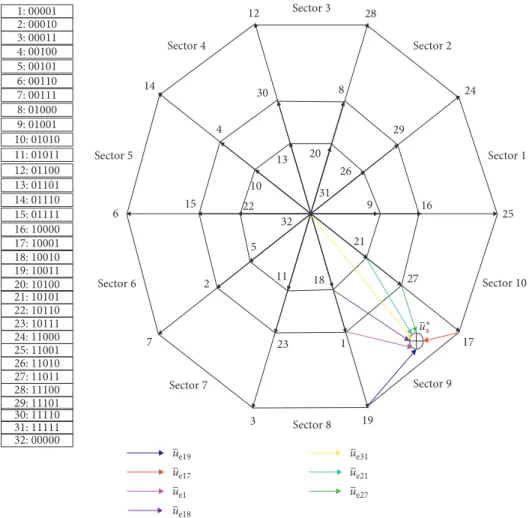
To investigate more about the selection mechanism of optimal voltage vector using the proposed cost function of (27) which based operation depends on achieving the minimum error between the actual applied voltage vectors and the reference voltage vectors, the voltage vectors dis- placement and their corresponding switching states are illustrated in Figure 5. It can be realized that, for a given reference voltage vectoru_s^∗located in sector 9, there will be seven possible voltage vectors which can achieve the control target (vector 19, vector 17, vector 1, vector 27, vector 18, vector 21, and vector 31 or 32). However, the optimal one that will be selected using the cost function of (27) is the vector that achieves minimum error (distance between the actual vector and reference vectoru_s^∗), which is here vector 17 that makes an error of u_e17. This process is performed without using any estimated quantities (in comparison with the MP DTC approach), which saves the computation time of the controller and reduces the switching losses of the inverter.

4. The Proposed Back-Stepping Observer

4.1. Mathematical Model of the Back-Stepping Observer.

The minimization of the error between the estimated and measured stator current values is the base principle upon which the back-stepping observer is designed. It is assumed that the components of the stator current are the outputs of the system which can be expressed by

y₁�x₁, y₂�x₂.

􏼨 (44)

Moreover, the model of the back-stepping observer is given by

􏽢_

x₁� −A􏽢􏽢x₁+K.A􏽢_r􏽢x₃+K.􏽢ω_mex􏽢₄+B.u_αs+V_α,

􏽢_

x₂� −A􏽢􏽢x₂+K.A􏽢_r􏽢x₄− K.􏽢ω_mex􏽢₃+B.u_βs+V_β,

􏽢_

x₃�L_mA􏽢_r􏽢x₁− A􏽢_rx􏽢₃− ω􏽢_me􏽢x₄,

􏽢_

x₄�L_mA􏽢_r􏽢x₂− A􏽢_rx􏽢₄+ω􏽢mex􏽢₃,

⎧

⎪⎪

⎪⎨

⎪⎪

⎪⎩

(45)

where

x₁ x₂ x₃ x₄

􏼂 􏼃^T�􏽨i_αs i_βs ψ_αr ψ_βr􏽩^T, A􏽢_r�A_r+ΔA_r�R_r

L_r+ΔR_r L_r , R􏽢_ϑ�R_s+L_m·μΔA􏽢_r,

A􏽢 � R􏽢_ϑ σL_s� R_ϑ

σL_s+L_m·μ·Δar

σL_s �A+ΔA, K� L_m

σL_sL_r, μ�L_m

L_r,

(46) where x􏽢_i is the estimate ofx_ifori∈{1,2,3,4}.

V_αandV_βrepresent the vector components that are built by the back-stepping strategy. In addition, all the parameters of the ﬁve-phase induction motor are considered to be known except the rotor resistance. The rotor resistanceR_ris considered as an uncertain parameter of nominal rotor resistanceR_rn.

4.2. Dynamic Model of the Estimation Errors. The equations of state errors are formulated as follows:

z_i�

z_y1�z_x

1

z_y2�z_x

2

⎡

⎣ ⎤⎦� x₁− x􏽢₁ x₂− x􏽢₂

􏼢 􏼣, (47)

z_ψ � z_x

3

z_x

4

􏼢 􏼣� x₃− 􏽢x₃ x₄− 􏽢x₄

􏼢 􏼣, (48)

where z_i and z_ψ represent the observation errors of the stator current and the rotor ﬂux, respectively.

Using (44), (47), and (48), the dynamic model of pre- diction errors is given by

_ z_x

1�K A_rz_x

3+ω_mez_x

􏼐 4􏼑+Δω_me􏽢x₄+ΔA_r L_mx₁− 􏽢x₃􏼁

􏼐 􏼑− V_α,

_ z_x

2�K A_rz_x

4− ω_mez_x

􏼐 3􏼑− Δω_mex􏽢₃+ΔA_r L_mx₂− x􏽢₄􏼁

􏼐 􏼑− V_β,

z__x

3� − A_rz_x

3+ω_mez_x

􏼐 4􏼑− Δω_mex􏽢₄+ΔA_r L_mx₁− x􏽢₃􏼁, _

z_x

4� −A_rz_x

4+ω_mez_x

􏼐 3􏼑+Δω_mex􏽢₃+ΔA_r L_mx₂− x􏽢₄􏼁,

⎧⎪

⎪⎪

⎨

⎪⎪

⎪⎩

(49) where the speed error is given by Δωme�ωme− ω􏽢me. In order to solve the problem of tracking and regulating the speed and rotor ﬂux and to overcome the diﬃculties that arise due to the unavailability of direct measurement of one of the state vector variables [30, 31], a nonlinear back- stepping observer is proposed.