Characterization of Precipitates in Steam Methane Reformer Tubes

Characterization of Precipitates in Steam Methane Reformer Tubes

by

Sakinah Binti Haris

Dissertation submitted in partial fulfillment of the requirements for the

Bachelor of Engineering (Hons) (Mechanical Engineering)

SEPTEMBER 2012

Universiti Teknologi PETRONAS Bandar Seri Iskandar

31750 Tronoh Perak Darul Ridzuan

i

CERTIFICATION OF APPROVAL

Characterization of Precipitates in Steam Methane Reformer Tubes

by

Sakinah Binti Haris

A project dissertation submitted to the Mechanical Engineering Programme

Universiti Teknologi PETRONAS In partial fulfillment of the requirement for the

BACHELOR OF ENGINEERING (Hons) (MECHANICAL ENGINEERING)

Approved by,

_________________________

(Dr. Azmi Bin Abdul Wahab)

UNIVERSITI TEKNOLOGI PETRONAS TRONOH, PERAK

September 2012

ii

CERTIFICATION OF ORIGINALITY

This is to certify that I am responsible for the work submitted in this project, that the original work is my own except as specified in the references and acknowledgements, and that the original work contained herein have not been undertaken or done by unspecified sources or persons.

_____________________

SAKINAH BINTI HARIS

iii ABSTRACT

Reformer tubes are critical components in steam-methane reformers and they are exposed to severe conditions of high temperature and pressure of endothermic hydrogen reforming reaction. The elevated temperature condition induced the reformer tube material to experience creep damage. It is vital to extend the life of the reformer tube in order to reduce the maintenance cost. The prolonged heating also developed carbide precipitations in the reformer tube. In this work, a study has been conducted to characterize the precipitates in the steam-methane reformer tube. The precipitates were characterized in terms of type and size, and the characterizations were then related to the conditions of an ex-serviced reformer tube.

iv

ACKNOWLEDGEMENT

At first, I would like to express my gratitude to Allah S.W.T that had made my final year project ran smoothly and end successfully. A greatest appreciation goes to Dr.

Azmi Abdul Wahab, my final year project‟s supervisor for his teachings, guidance, supports and supervision towards completing my project. From such project, I have gained valuable knowledge and deepened my comprehension regarding the microstructure characterization and its behavior which I believe could be useful in my future application and contribution. A lot of explanation and support has been given by my supervisor to get through the hardest part of completing the project. In the hard times, I have learnt values to always be positive, patient, determine and persevere to achieve the goal. Also, special thanks to my family and colleagues for their moral support, inspiration and advice throughout the period. May all of you gain His Blessings and His Love.

v TABLE OF CONTENTS

CERTIFICATION OF APPROVAL . . . . . i

CERTIFICATION OF ORIGINALITY . . . . . ii

ABSTRACT . . . . . . . . . iii

ACKNOWLEDGEMENT . . . . . . . iv

LIST OF FIGURES . . . . . . . . vii

LIST OF TABLES . . . . . . . . ix

CHAPTER 1: INTRODUCTION . . . . . 1

1.1 Background of Study . . . . 1

1.2 Problem Statement . . . . 3

1.3 Objectives of Study . . . . 3

1.4 Scope of Study . . . . 3

CHAPTER 2: LITERATURE REVIEW . . . . 4

2.1 Steam Methane Reformer . . . 4

2.2 Steam Methane Reformer Tubes . . . 5

2.3 Carbide Precipitations in Reformer Tubes . 6 2.4 Characterization of Carbide Precipitates in Austenitic Stainless Steel . . . . 8

2.5 Quantitative Image Analysis . . . 13

CHAPTER 3: METHODOLOGY . . . . . 16

3.1 Project Framework . . . . 16

3.2 Imaging Tools . . . 17

3.3 Preliminary Research . . . . 18

3.4 Collection and Organization of Data . . 18

3.5 Data Processing . . . 19

vi

3.5.1 Cropping image . . . . 19

3.5.2 Highlighting precipitates features . 20

3.6 Analyze Data . . . 21

3.6.1 Area threshold . . . . 21

3.6.2 Area measurement . . . 23

3.6.3 Three Dimensional (3D) reconstruction and

visualization . . . 25

CHAPTER 4: RESULT AND DISCUSSION . . . 27

4.1 Result . . . 27

4.2 Effect of different service temperature on the precipitation

formation . . . 27

4.3 Service condition of the sample XC and XH . 32 CHAPTER 5: CONCLUSION AND RECOMMENDATION . 37

5.1 Conclusion . . . 37

5.2 Recommendation . . . 38

REFERENCES . . . . . . . . 39

vii

LIST OF FIGURES

Figure 1.1 The effect of exceeding the design temperature on the

expected life of HK-40 alloy reformer furnace tubes. . 2 Figure 2.1 Scheme of a hydrogen production system comprising a

steam-methane reformer . . . 5

Figure 2.2 Schematic view of a top fired reformer furnace . . 6 Figure 2.3 Microstructure of as-cast and after annealing alloys . . 9 Figure 2.4 Multiphase aggregated carbides on the grain boundaries after

the annealing and results of quantitative microprobe analysis

of the precipitates and the matrix (%) . . . . 10 Figure 2.5 Backscatter electron (BSE) image of ex-service reformer tube

and the corresponding EDS spectra of precipitates A, B, and C 12 Figure 2.6 XRD Spectrum of reformer tube precipitates. M23C6, NbC

and TiC peaks are indicated . . . 12 Figure 2.7 Three dimensional reconstruction can be obtained by

systematic thinning of specimen. . . 15 Figure 3.1 The flow chart of project methodology . . . 16 Figure 3.2 The NIH ImageJ user window. . . . . 18 Figure 3.3 Process of cropping image from the raw stack images.

a) 664 x 470 pixels rectangular selection of stack images

b) with 50% zoom. b) Cropped image viewed in 100% zoom. 20 Figure 3.4 Image processing. a) Type of precipitates was determined.

b) Highlighted Cr23C6 precipitates features.

c) Highlighted NbC precipitates features.

d) No presence of TiC to be highlighted. . . . 21 Figure 3.5 Command windows to adjust image with color threshold. . 22 Figure 3.6 Particle regions threshold for the first layer of sample K0; Cr23C6. 23 Figure 3.7 Re-scaling the measurement unit from pixels into µm. 23 Figure 3.8 Command to analyze particles threshold. . . . 24 Figure 3.9 Result presentation of analyzed particle threshold; masks of

particles, table of results, and result summary. . . 24

viii

Figure 3.10 Microsoft Excel spreadsheet used to tabulate the entire

stacks of analyzed particles. . . 25 Figure 3.11 The masks images of sample K0 were re-stack and saved in

different TIFF file. . . 26

Figure 3.12 The volume viewer showing the distributions of Cr₂₃C₆ of sample

K0 in isometric view. . . . 26

Figure 4.1 Graph of mean volume of precipitate against the service

temperature. . . 28

Figure 4.2 Optical image of Sample K1 at 200X magnification. . . 29 Figure 4.3 Optical image of Sample K2 at 200X magnification. . . 30 Figure 4.4 Optical image of Sample K3 at 200X magnification. . . 30 Figure 4.5 Optical image of Sample K0 at 200X magnification. . . 31 Figure 4.6 The mean volume of Chromium Carbide precipitates against

the service temperature . . . 32 Figure 4.7 The mean volume of Niobium Carbide precipitates against the

service temperature . . . 33

Figure 4.8 The mean volume of Titanium Carbide precipitates against the

service temperature . . . 33

Figure 4.9 The linear regression of mean volume of Cr23C6 with the

operating temperature . . . 35

Figure 4.10 The linear regression of mean volume of NbC with the

operating temperature . . . 35

Figure 4.11 The linear regression of mean volume of TiC with the

operating temperature . . . 36

ix

LIST OF TABLES

Table 2.1 Nominal Composition of Principal Alloys Used for Tubular

Tubular . . . 7

Table 2.2 Comparison of selected properties of human and computerized vision system when applied in metallography . . 13 Table 3.1 Detail service condition of the samples . . . 18 Table 3.2 Chemical Composition of Schmidt + Clemens CA4852 micro

alloy material . . . 19

Table 4.1 Data tabulation of average particle size to the service temperature 27

Table 4.2 XH and XC tabulated data . . . 34

Table 4.3 Table for calculated temperature based on linear equations

produced in graphs . . . 34

1

CHAPTER 1 INTRODUCTION

1.1 Background of Study

Reformer furnaces are used in petrochemical industry to produce hydrogen, carbon monoxide and carbon dioxide. More recently, with the increase of hydrogen gas demand, reformer furnaces are widely used for the large scale production of hydrogen gas. Reforming process is also well known for its economical way of production [1].

With the catalytic reactions that occur, the reactants – hydrocarbons and steam are converted into hydrogen and carbon dioxide [2]. The following are the general reactions of the process in the reformer furnaces.

C_nH_m+ nH₂O nCO + (m/2 + n) H₂ (1) CO + H₂O CO₂ + H₂ (2)

Most reformer furnaces undergo Steam-Methane Reforming (SMR). However, other C_nH_m, hydrocarbons such as ethanol, propane or even gasoline are also used in reforming process of hydrogen [3]. The above endothermic reaction is conducted in high temperature of a steam reformer furnace with temperature exceeding 1073K for the reaction to take place. The steam reformer furnace contains numerous vertically mounted tubes filled with catalyst in which they are continuously heated to achieve the required temperature. Thus, the critical components of a reformer furnace are the reformer tubes themselves due to the severe heat exposure during the service [2].

Steam reforming tubes are usually made of centrifugally cast austenitic stainless steel [4]. It is designed with normal life of 100,000 hours, however, in real service conditions the life varies depending on the service condition and the characteristic of materials used [5]. Upon the severe heating of the reformer tube, the microstructure of

2

the cast stainless steel will change substantially resulting in a change in mechanical properties. The microstructural changes however, could be used to determine the actual wall temperature and also other mechanical attributes of the material itself [6].

Research has confirmed that, the most important damage mechanism leading to the failure of the reformer tube is creep, and it is shown in Figure 1.1, the effect of increased local temperature could cause a dramatic reduction in life. From the figure, it is shown that the further the difference between average temperature from its base design temperature, the lesser the percentage of expected tube life of an alloy [7].

Most of the existing study illuminates the variations of microstructure and mechanical properties of the tubes during the operation along with time and usually relates in determination of remaining lifetime of the tubes.

Figure 1.1: The effect of exceeding the design temperature on the expected life of HK-40 alloy reformer furnace tubes [7].

However, research has also found that, the presence of secondary precipitates as an effect of the heating inside the reformer tubes may contribute to creep strengthening of the material and may cause tube failure [8]. Therefore, the purpose of this project was to investigate the relationship between the precipitations in reformer tube with the service condition.

3 1.2 Problem Statement

Reformer tubes are the critical components of a reformer furnace due to severe heat exposure during service. The material that is generally used for reformer tubes is a type of special cast alloys with increased creep strength, greater resistance to overheat, and longer tube service life [8]. The heating process during the operationwould change the material microstructure such thatcarbide precipitations form at the interdendritic region [9]. It would be of great intent to relate the characterization of these precipitates to the service condition of the material.

1.3 Objectives of Study

The main objectives of this project are:

I. To characterize themicrostructure of the precipitate that form in the ex-service reformer tube by using metallography and microscopy techniques.

II. To correlate between the microstructural features of precipitates to the service condition of the tube.

1.4 Scope of Study

In this project, all the samples of ex-serviced reformer tubes were obtained from MethanexKitimat Plant, Canada. The reformer tube material is Schmidt + Clemens CA4852 micro alloy from Spain. The samples data are given the nomenclature and operating conditions section. Total five samples were analyzed which were randomly sectioned out at different length of the same reformer tube. Three of them were provided with operating conditions information while the remaining two were only stated to be in overheated service condition and at normal service condition respectively.

Characterization process will involve analysis of optical microscopy data obtained from the metallographic sample prepared. Characterization of precipitates will be limited to Chromium Carbide (Cr23C6), Niobium Carbide (NbC) and Titanium Carbide (TiC) precipitates only. The amount and size of the precipitates will be related to the service conditions experienced by the tube.

4

CHAPTER 2

LITERATURE REVIEW

2.1 Steam Methane Reformer

In petrochemical industry, Steam-Methane Reforming (SMR) Process has been extensively used in production of hydrogen from fossil fuels, in which the methane reacts with steam to produce a mixture of hydrogen (H2), carbon dioxide (CO2) and carbon monoxide (CO) [10]. A mixture of CO₂ and H₂ then is used to produce chemical products with high added values such as hydrocarbons and oxygenated compound. It is a very energy intensive process due to highly endothermic reaction which is well suited for processes requiring a H₂-rich feed like ammonia synthesis and petroleum refining process [9].

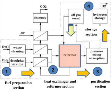
Figure 2.1 briefly describe the flow of hydrogen production process comprising steam-methane reforming process inside the reformer. The steam reformer is where the high-energy endothermic reaction of reforming process takes place. Firstly, the fuel preparation section takes place to cleanse the feed water and desulphurize the methane gas before they are mixed into the reformer furnace. In the second section, there are two main processes that occur; steam-methane reforming and water-gas shift reaction.

1. Steam-methane reforming

In steam-methane reforming methane reacts with high temperature steam (970 – 1100K) at 3.5MPa in the presence of a catalyst to produce CO and H2.

Steam-methane reforming is endothermic in which heat must be supplied for the reaction to occur [11].

CH₄ + H₂O CO + 3H₂ ∆H°298 = + 241 kJ/mol (3)

5 2. Water-gas shift reaction

In this phase, exothermic reaction of CO with H2O (steam) is then carried out to produce H₂ at 470 – 820K [3]. Conventionally, the process is performed in multi-tubular fixed-bed reactors in the presence of a metal catalyst [12].

CO + H₂O CO₂ + H₂ ∆H°298 = -41.1 kJ/mol (4)

In the purification section, pressure swing adsorption is commonly used to remove CO₂, water, methane and CO from the off gas leaving essentially the pure H₂ [11].

The unwanted gases would then be recycled to the reformer through off-gas vessel.

Figure 2.1: Scheme of a hydrogen production system comprising a steam-methane reformer. [1]

2.2 Steam-Methane Reformer Tubes

The design of steam-methane reformer tubes has greatly improved over the past 30 years. The alloys and manufacturing process development has contributed to meet the severe requirements of the reformer tubes, which are operating in the radiation zone and in the hot reaction gas outlet. The use of catalyst such as Nickel (Ni) also provide lower temperature reactions thus aiding to equalize the need of increase temperature

fuel preparation section

heat exchanger and reformer section

purification section storage section

6

and pressure to achieve further increases in production and reformer furnace efficiency [7].

Figure 2.2: Schematic view of a top fired reformer furnace [7].

A steam reformer is made up of catalyst-filled reformer tubes arrays arranged in the form of two vertical walls. The number of columns varies between 15 and 200;

depend on the number and size of the walls. Most of the reformer furnaces are of the top-fired type at which the burners are dispersed rows on both side of columns.

Charge will be given through the inlet pigtails above the roof of radiation chamber and the reformer tubes column is suspended with use of counterweights. The producing gas will then leave the column through the outlet pigtails connecting to outlet manifold [7].

2.3 Carbide Precipitation in Reformer Tubes

On the basis of API 530, the design of nominal life of a reformer tube should be 100,000 hours however it depends on the actual operating conditions and characteristic of the particular tube material. Owing to the severe operating conditions, reformer tubes are typically made of ACI HK40 (0.4 wt%C – 25 wt%Cr –

7

20 wt%Ni) and ACI HP40 (0.4 wt%C – 25 wt%Cr – 35 wt%Ni) [4]. The dimensions of the reformer tubes manufactured vary between 10 and 15m in height, 100 to 200mm diameter, and 10 to 25 mm wall thickness [4].

Since early 80s, modern alloys such as the HP types have been made available in which it contributes to strength and corrosion resistance at high temperature. Table 2.1 below presents the nominal composition of principal alloys used for reformer tubes manufactured by Schmidt + Clemens (S+C) & Co. KG [9].

Table 2.1: Nominal Composition of Principal Alloys Used for Tubular Reformers [9].

As presented by Schmidt + Clemens (S+C) & Co. KG, during the service of reformer tube, a significant number of full thermal and pressure cycles caused by plant start- ups and shut-downs happens throughout the process. This condition can be very damaging and could accelerate creep cracking. For reformer tubes, which are working under severe condition, centrifugally cast material, are mostly favored [9].

During the metal casting of the tube material, primary eutectic-like carbide network formation plays important role in preventing grain boundary sliding [13]. However, at the early stages of SMR process, precipitation of carbides occurs in reformer tubes.

This would reduce the strength and cause embrittlement of materials due to coalescence and coarsening of carbides. Further degradation could lead to creep damage, micro cracking and final propagation of macro-cracks [5]. The carbide formation consists of austenitic dendrites surrounded by eutectic carbides in the interdendritic region. This carbide formation is also known as secondary precipitation.

Studies have been done proving that better creep properties have been attributed to the morphological modification and the presence of more stable phases during the long-

8

term service. The recent modification of adding niobium-plus-titanium has promoted the fragmentation of the as-cast microstructure and partially replaces the chromium carbide into more stable ones. It is in the form of a fine-distribution of cube-shaped chromium carbides that it should act to restrict the motion of dislocations [13]. This proves that alloys do rely upon creep strengthening by the formation of more stable carbides in the microstructure especially during a long-term high temperature service [9].

2.4 Characterization of Carbide Precipitates in Austenitic Stainless Steel.

Based on the microstructure study of the as-cast and annealed austenitic steels, findings have shown that in the as-cast state, the microstructure comprise of austenitic matrix and primary precipitates of carbide which are present at the boundaries of grains and in the interdendritic areas.

Figure 2.3 shows the comparison of microstructure before and after the alloys were annealed. Alloys 1 and 2 above show the effect of titanium and niobium addition, respectively. It is proven that annealing significantly changed the microstructure of the alloys. Also alloys 1 and 2 show changes at and around the boundaries of austenite grains with large amounts of fine secondary precipitates at the matrix interfaces.

9

Figure 2.3: Microstructure of as-cast and after annealing alloys. [14]

10

Figure 2.4: Multiphase aggregated carbides on the grain boundaries after the annealing and results of quantitative microprobe analysis of the precipitates and the

matrix (%) [14].

Figure 2.4 above shows the confirmed microstructure of carbide elements in the alloys tested. The microanalyses were performed by using microprobe analysis. The results are concluded as follows [14]:

Alloy 1: Precipitate 1 is chromium carbide of M23C6type; precipitate 2 is TiC carbide while the areas 3 and 4 are rich in nickel, silicon and titanium. It is proven that not all titanium is used in formation of the TiC during solidification process.

11

Alloy 2: Precipitate 1 is probably NbC carbide; precipitate 3 is chromium carbide M23C6 type. The chemical analysis in area 2 indicates rich of silicon, nickel, and niobium.

Alloy 3: Precipitates 1 and 3 are NbC carbides alloyed with titanium, precipitate 5 is TiC carbide alloyed with Nb. The area 4 is probably a secondary solution of both Ti and Nb carbide. TiC –NbC complex and the NbC carbides are denoted by number 2.

It was rich in silicon, nickel, niobium and titanium, Pheses rich in silicon, nickel and niobium in austenitic alloys reported earlier in other findings [15,16], the phase has been named “G” phase and the formula of Nb6Ni16Si7 has been attributed.

In a previous research identification of precipitates that form in the same reformer tube originated from Methanex Kitimat Plant, Canada has been made. Precipitates A and B as labeled in Figure 2.5(a), appeared as light blue and grey respectively, and were usually found along the grain boundaries. From the EDS result shown in Figure 2.5(b), precipitates A show the highest content of chromium elements and it was confirmed in a XRD method that the precipitate A is Cr23C6 as illustrated in Figure 2.6. The EDS confirmed precipitates B and C to be NbC and TiC respectively as shown in Figure 2.5(c) and (d). Precipitate C appeared as orange-brown and usually resided intragranularly. In the sample, there is also presence of void, which appeared next to precipitate A [3].

12

Figure 2.5: Backscatter electron (BSE) image of ex-service reformer tube and the corresponding EDS spectra of precipitates A, B, and C [3].

Figure 2.6: XRD Spectrum of reformer tube precipitates. M23C6, NbC and TiC peaks are indicated [3].

b) EDS spectrum of precipitate A;

a) BSE image of as-cast tube;

d) EDS spectrum of precipitate C;

c) EDS spectrum of precipitate B;

13 2.5 Quantitative Image Analysis.

In material characterization, quantitative image analysis is developed to extract meaningful information from microstructure images captured. It can be assessed by human manually or automatically conducted by machine that has been allowed for the construction of personal-computer-based digital image analyzers. Nevertheless, this enormous progress of the machine has been implemented on a limited scale due to introduction of user-friendly, icon-based software that can be applied on any computer device. People are afraid of using computerized tools in metallographic laboratory and declare that the machine would never do as good and thorough analysis as an experienced metallographic practitioner. The comparison between the traditional and computer-aided image analysis based on certain properties is shown in Table 2.2.

Table 2.2: Comparison of selected properties of human and computerized vision system when applied in metallography [15].

14

Image is a representation of an object produced by lens or mirror system. The image is a data set, stored in a computer memory or in a digital file that can be displayed on screen or printed for human observation. The elementary unit of a digital image is called pixel. When an image is displayed in a computer monitor, it is a mosaic of pixels. The location of each pixel is defined by the image format (Tagged Image File Format or TIFF, BMP, Joint Photographic Expert Group or JPEG, etc.). The body of the digital file contains information concerning pixel intensity or color [15].

Image processing is part of image analysis. It is a process of data transformation in which the initial data set is an image or a collection of images and the final, resulting data set is also an image or a collection of image. Image processing also can be called digital imaging, as is done within this volume. The aim of image processing is to highlight the features under investigation or to suppress the unwanted features. The process of image acquisition is usually interpreted as the introductory part of image processing. Image processing, in image analysis – the computer modification of a digitized image on a pixel-by-pixel basis is to emphasize certain aspects of the image.

The final step of image analysis can be in various characters such as characterizing the grain size [15].

Digital measurement are the core of quantitative image analysis as to determine the size distribution. According to ASTM, estimation of the mean object section area can be calculated using the formula below,

𝑎 = _𝑁^𝐴𝐴

𝐴 (5)

where𝑎 is the mean object area, 𝐴_𝐴is the area fraction of the objects analyzed, and 𝑁_𝐴 denotes the number of objects per unit section area.

To characterize sructural parameters of any microstructure, they are four characters that are necessary to describe its properties which are amount, size, shape and spatial distribution of all the phases. However of all, distribution is the most difficult to quantify. Any material built of two or more phases is non-homogenous. When it is oberseved at very high magnification only the phases can be distinguished clearly. On

15

the other hand, when the microstructure is observed by human eye, it can seems to be homogenous. Therefore, the result of homogeneity quantification only applicable at high magnification. This situation can be improvised by using three-dimensional (3- D) images. The oldest technique for obtaining 3D data is to prepare a series of polished sections with a systematic shift in direction perpendicular in z-direction.

There are some drawbacks in such method where it is practically impossible to ensure same step in z-direction and the resolution in this direction significantly lower than the section plane. Despite of these drawbacks, it is allowed for evaluation of real 3D shapes of grains [15].

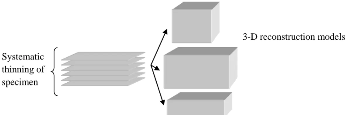
From this systematic thinning of the specimen, the subsequent 3-D reconstruction can provide real shape and arrangement of features that are not available in any other methods. In contrast, image analysis packages or software equipped with 3-D analysis tools allow for filtering, binarization (two form 2 values of pixel) and measurement similar to those used in 2-D image analysis. Unfortunately, such ability requires huge computing power and computer memory to process the data. There is a software that could meet such requirements namely NIH ImageJ application software. It is known as the fastest image analyzer packages written in JAVA which is user-friendly and are now used worldwide. It is significance to do 3-D analysis as it offers the ability to obtain real, volumetric distribution of some features in the analyzed microstructure.

Nevertheless, this 3-D has its own limitation that it is practically impossible to detect grain boundaries. Therefore, this techniques is suitable for assesment of porosity and homogeneity of phases in a microstructure. Figure 2.7 illustrates the 3-D reconstruction from the systematic thinning of specimen [15].

Figure 2.7: Three dimensional reconstruction can be obtained by systematic thinning of specimen.

3-D reconstruction models Systematic

thinning of specimen

16

CHAPTER 3 METHODOLOGY

3.1 Project Framework

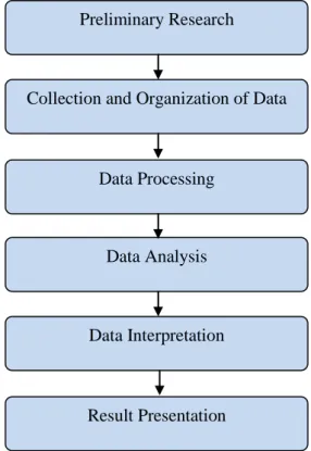
The characterization of precipitates in this project has been conducted based on data obtained from prepared metallographic samples. Figure 3.1 shown below is the general step of conducting the project.

Figure 3.1: The flow chart of project methodology.

Samples for this work have been previously prepared metallographically. Optical images of the microstructure had been obtained at various location of the reformer tube. This project began with data organization to arrange the images according to their respective group samples. Next, the data have been processed by identifying the

Preliminary Research

Collection and Organization of Data

Data Processing

Data Analysis

Data Interpretation

Result Presentation

17

respective precipitates from the images. The sizes of precipitates for each of the samples were analyzed by means of area measurement and 3-D reconstruction. All the samples have undergone same process. Finally, the result obtained were plotted on the graph for further interpretation and comparison between the known service condition samples with the unknown service condition to locate and determine the service condition experienced by the samples.

3.2 Imaging Tools

NIH ImageJ software was used throughout the image analysis. NIH ImageJ is an open-source software that their Java source codes are freely available in public domain and no license is required. Since it is written in Java, it allows running on Linux, Mac OS X and Windows, in both 32-bit and 64-bit modes. It has large and knowledgeable worldwide user community. It is the world‟s fastest pure Java image processing program that it can filter a 2048 x 2048 image in 0.1 seconds, about 40 million pixels per second. It can be opened and saved in all supported data types 8-bit grayscale or indexed color, 16-bit unsigned integer, 32-bit floating point and RGB as TIFF or as raw data. Other file formats are GIF, JPEG, BMP, PNG, PGM, FITS and ASCII. The zooming tools (1:32 to 32:1) are provided and all analysis and processing functions are able to work at any magnification factor [16].

Selections can be made by creating rectangular, elliptical or irregular area selection.

To make irregular area selection, lines and point selection is created. Next selection is edited and automatically created using the wand tool. Drawing, filling, filtering or measuring of selection can be easily conducted through the program. For image enhancement, this software supports smoothing, sharpening, edge detection, median filtering and thresholding on both 8-bit grayscale and RGB color images. It is also can interactively adjust brightness and contrast of 8, 16, and 32-bit images. Other functions such as geometric operations, image analysis, image editing, and color processing are also featured in this ImageJ software. For geometric operations, the image can be cropped, scaled, resized and rotated. It can perform image analysis such as measure area, mean, standard deviation, min and max of selection image. It also uses real world measurement such as SI units. To cut, copy or paste images or selections by using AND, OR, XOR or “Blend” modes. It provides display a "stack"

18

of related images in a single window. The process applies to the entire stack using a single command [16].

Figure 3.2: The NIH ImageJ user window [16].

3.3 Preliminary Research

Before conducting the experimental work, background of Steam-Methane Reformers were studied. The sources of information were obtained from articles, textbooks, journals and company websites. It is important to understand the operation of steam- methane reformer to relate the operation principles with carbide precipitations. At this stage the theory of precipitates formation due to annealing process also has been reviewed as well as characterization techniques done through researches.

3.4 Collection and Organization of Data

There are six data samples sectioned out from the same type of reformer tube used in this project work. Three of them, sample K1, K2 and K3 were all taken randomly with various operational conditions of their temperature and pressure in service as shown in Table 3.1 below while the remaining two samples were only known for its general serviced temperature under overheated or normal temperature. Sample K0 is the as- cast sample.

Table 3.1: Detail serviced condition of the samples.

Sample Service hours

(hr)

Distance from top flange (m)

Temperature in service

(°C)

Pressure in service

(MPa)

K0 N/A N/A N/A N/A

K1 90,000 12.5 878 – 888 1.82

K2 90,000 9.9 867 – 886 1.91

K3 90,000 2.4 775 – 848 2.16

XH 90,000 Unknown Overheated

temperature

Unknown

XC 90,000 Unknown Normal

temperature

Unknown

19

The chemical compositions of the Schmidt + Clemens CA4852 micro alloy reformer tube samples were listed in Table 3.2.

Table 3.2: Chemical Composition of Schmidt + Clemens CA4852 micro alloy material [17].

Chemical

Composition C Si Mn Cr Ni Nb Ti Fe

Mass percentage 0.45 1.50 1.00 25.0 35.0 1.50 Additions Balance

The data obtained was in the form of TIFF (Tagged Image File Format) files of optical microscopy images with 200X magnification and had been aligned previously.

Each sample was provided with 50 images of its consecutive layers after polishing with approximate depth of 0.5µm each. By using the ImageJ software the images were orderly stacked and was saved as one TIFF file. The same procedure was done to the other four samples. The „image stack‟ allows the images to be displayed and processed through the same window. For every consecutive layer, the changes of microstructure are approximately 0.5µm depth.

3.5 Data Processing

Data processing is the image processing stage in which the initial images were transformed into other type of image. The aim of this image processing is to highlight the image of respective precipitates; Chromium Carbide, Niobium Carbide and Titanium Carbide. Each stacked image sample has undergone three modification processes and the precipitates were selected traditionally with reference from preliminary research regarding the precipitates features. The selected regions were the coarse precipitates and were kept constant for the whole layers to reduce errors during the analysis.

3.5.1 Cropping image

The raw „image stack‟ were then cropped randomly into 664 x 470 pixels image. It is randomly cropped at the region with well-defined shape of precipitates as well as no external disturbance such the superimposed indentations image. Figure 3.3 shows the image is cropped from raw images at 50% zoom and after that appeared in 100%

zoom.

20

Figure 3.3: Process of cropping image from the raw stack images. a) 664 x 470 pixels rectangular selection of stack images with 50% zoom. b) Cropped image viewed in

100% zoom.

3.5.2 Highlighting precipitates features

Before the image could be analyze with area measurement and 3-D reconstruction, the image stacks were processed in which the features of interest were highlighted. The process is conducted by using NIH ImageJ paint tools where the background colors were picked to erase the non-interest features. The same highlighting process was done to the entire series of images to generate a new stack of images with feature of interest only.

a) b)

21

Figure 3.4: Image processing for sample K0. a) Type of precipitates were determined.

b) Highlighted Cr23C6 precipitates features. c) Highlighted NbC precipitates features.

d) No presence of TiC highlighted.

3.6 Analyzing Data

Data analysis has been done on basis of quantitative image analysis. The sizes of precipitates from the images captured were measured and the resulting size is defined by the estimated volume of precipitates in the samples. The mean area of stacked images is measured and each of the images in the stack would undergo same process.

3.6.1 Area threshold

After the precipitates features of interest have been processed, the selected region of precipitates would undergo color thresholding since the automatic particle analysis requires the image to be a „binary‟ image. The software needs to know exactly where the edges are to perform morphology measurements. A „threshold‟ range was set and

Cr23C6

NbC

a) b)

d) c)

22

pixels in the image whose value lies in this range are converted to red as requested while pixels with values outside this range are converted to white.

The thresholding process is a bit more complicated as each of hue, saturation and brightness channels requires different threshold range as described shown Figure 3.6.

Manual thresholding requires human interpretation on which area were being thresholded. Therefore to improve the quality of thresholding, the images were unstack and thresholded individually otherwise the calculated threshold of the currently displayed slice will be used for all slices. The images should also been re- scaled to get the measurement in unit of micrometer as in Figure 3.7. It would be useful in area measurement in the next stage of image analysis.

Figure 3.5: Command windows to adjust image with color threshold.

23

Figure 3.6: Particle regions threshold for the first layer of sample K0; Cr23C6.

Figure 3.7: Re-scaling the measurement unit from pixels into µm.

3.6.2 Area measurement

Using analyze tool of NIH ImageJ, the analyze particle command has been selected to counts and measure the area of threshold image. Figure 3.8 shows the command windows of the process. The analysis was done by scanning the selected particle within the range of threshold. The result obtained was presented in unit of µm².

24

Figure 3.8: Command to analyze particles threshold.

Figure 3.9: Result presentation of analyzed particle threshold; masks of particles, table of results, and result summary.

Figure 3.9 above shows the masks, results and summary of the analysis as requested.

The summary window presented the counts, total area, average size, percentage and mean area of the analyzed particles. Each of the images would produce their own measurement information. Later, the collection of information was tabulated in the Microsoft Excel spreadsheet. The mean area calculated was then multiplied with the number of stacking images in which each layer equals to 0.5µm depth.

25

Mean Area Sample = Total Area of precipitate in 50 layers (6) 50 layers

Mean Volume of sample = Mean Area Sample x 50 x 0.5 µm (7)

Figure 3.10: Microsoft Excel spreadsheet used to tabulate the entire stacks of analyzed particles.

3.6.3 Three Dimensional (3D) reconstruction and visualization

To reconstruct and visualize the three dimensional (3D) of stack images, all the masked images were re-stacked and were saved into a new TIFF image file before it is to perform the reconstruction function. Then 3D Plug-in was used to generate Volume Viewer (See Figure 3.11). The volume viewer windows would pop out as in

26

Figure 3.12. In this project, the volume has been processed in slow resolution and is presented in isometric view.

Figure 3.11: The masks images of sample K0 were re-stacked and saved in different TIFF file.

Figure 3.12: The volume viewer showing the distributions of Cr₂₃C₆ of sample K1 in isometric view.

27

CHAPTER 4

RESULTS AND DISCUSSION

4.1 Results

The image analysis has provided significant quantitative analyses of the carbide precipitates formation in the reformer tube. The influence of service temperature and pressure to the carbide precipitation has been observed and presented in tables and graphs to relate between the service conditions and the carbide precipitates characteristics. Various literature sources have been reviewed to discuss the findings and to formulate a conclusion.

4.2 Effect of different service condition on the carbide precipitation formation.

Table 4.1 below shows the tabulated data for the variation of service temperature and service pressure exposure and their relation to the average particle size of precipitates formed.

Table 4.1: Data tabulation of average particle size to the service temperature.

Sample

Service Temperature

(ºC)

Mean Volume (10³ µm³) Cr23C6 NbC TiC

K0 N/A 57.652 21.762 0.00

K1 888 87.992 29.719 5.778

K2 886 74.911 26.732 1.956

K3 848 73.799 25.032 0.067

28

Figure 4.1: Graph of mean volume of precipitate against the service temperature.

As shown in Figure 4.1, the mean volume of chromium carbide, Cr₂₃C₆ precipitates is increasing as the service temperature increase. At 888 ºC, the service temperature of Sample K1, the mean volume of chromium carbide precipitates is the largest compared to the other lower temperature samples. Figure 4.2 shows large chromium carbide precipitates that formed at the grain boundaries. However, at certain higher temperatures, secondary precipitation is expected to happen in which it can be seen clearly as a dispersion of fine particles within austenitic matrix [2]. In sample K1, there is little presence of secondary precipitates that it is likely because of chromium depletion and outward diffusion related to the development of chromium-rich oxide layer [2]. During the degradation, the carbides detached away from the grain boundaries. Isolated voids were also apparent presumably due to Kirkendall effect.

Kirkendall effect describes the phenomenon when two solids diffuse into each other at different rates. The atoms of the solids don‟t change places directly; rather diffusion occurs where voids are left opened [18].

K1

K2 K3

K2 K1 K3

K1 K2 K3

0 10 20 30 40 50 60 70 80 90 100

840 850 860 870 880 890

Mean Volume (103µm3)

Service Temperature (°C)

M23C6 NbC TiC

K0 K0

K0

29

Figure 4.2: Optical image of Sample K1 at 200X magnification.

At service temperature of sample K2, 886ºC the mean volume of Cr23C6 precipitates, abruptly becomes smaller than in K1 sample. It is believed that this is caused by the precipitation of fine secondary carbide. As can be seen in Figure 4.3, an optical image of sample K2 shows that there is presence of fine precipitates away from the grain boundary labeled as secondary precipitates. While at lower temperature of 848 ºC, massive precipitation of fine secondary precipitates has caused the remaining mean volume of primary precipitates become smaller as presented in Figure 4.4.

As have been mentioned in section 3.5 previously, during highlighting the features of carbide precipitates, only the large and significant primary carbides were selected.

The large carbide precipitates is likely to have formed during the early stage of precipitation. Therefore, the increase in temperatures in sample K2 and K3 is the reason chromium carbide precipitates were detected less in the microstructure. At 886ºC, the secondary precipitates occur but at lower amount compared to 848ºC as shown in Figure 4.4.

Voids

Cr23C6

NbC TiC

30

Figure 4.3: Optical image of Sample K2 at 200X magnification.

Figure 4.4: Optical image of Sample K3 at 200X magnification.

It has been reported that NbC precipitates is not stable in the range of temperature between 700 and 900 ºC. From Figure 4.1, at 888 ºC the niobium carbide precipitates were slightly bigger than at 848ºC and 886ºC, it may due to the vacancy diffusion of niobium elements to the carbon elements during chromium depletion to form secondary precipitates or is there any case of chromium oxide formation. At higher temperature of 888ºC or even at 886ºC, niobium carbide is unstable, and there is possibility to transform into a nickel-niobium silicide, Nb₆Ni₁₆Si₇ which some study regarded it as G-phase [2]. However, the G-phase could best be identified by using X- ray diffraction spectra and are not easily detected by observation through optical images.

Cr23C6

NbC

TiC Voids

Secondary precipitates

Cr23C6 NbC

TiC

Secondary precipitates Voids

31

Titanium carbide precipitates are larger at 888ºC temperature compared to at service temperature of 848ºC and 886ºC. The coarsening rate varies with the composition in material with TiC. If there is a presence of Cr and Ni, the coarsening will become slightly faster. This is because Ni is a strong austenite stabilizer. A study also proved that the coarsening rate increases with increasing temperature [19]. This effect is caused both by increase in the diffusion rates and the increase in solubility of the Titanium element in the matrix. However, the slight decrease of the Titanium carbide average size at 886ºC is may due to the formation of intermetallic phase rich in silicon, nickel, titanium that is very likely to be the G phase denoted as M6Ni16Si7

[20].

Figure 4.5: Optical image of Sample K0 at 200X magnification.

The microstructure of the as-cast sample which is sample K0 consisted of an austenitic matrix and a network of two types of primary carbides which are chromium and niobium as shown in Figure 4.5. No titanium carbides formation has occurred.

The shapes of primary carbides are finer compared to the ex-serviced samples as in K1, K2, and K3 where the primary carbides coarsen with increase in servicing temperature [3]. This is the reason the mean volume of carbide precipitates are always the lowest in the as-cast sample.

Cr23C6

NbC

32

4.3 Service Temperature of the sample XH and XC.

The prediction of two unknown samples XC and XH will be made based on the size comparison of all three precipitates - Chromium Carbide, Niobium Carbide and Titanium Carbide, and comparing them to the data for K1, K2, and K3 samples. To make the comparisons more reliable, the data has been plotted into regression model as presented in Figure 4.6, 4.7, and 4.8.

Figure 4.6: The mean volume of Chromium Carbide precipitates against the service temperature.

y = 0.208x - 103.5

50 55 60 65 70 75 80 85 90 95 100

845 850 855 860 865 870 875 880 885 890

Mean Volume (103µm3)

Service Temperature (°C)

Mean Volume of CrC Precipitates (10³µm³) VS Service Temperature (°C)

33

Figure 4.7: The mean volume of Niobium Carbide precipitates against the service temperature.

Figure 4.8: The mean volume of Titanium Carbide precipitates against the service temperature.

y = 0.084x - 46.83

20 22 24 26 28 30 32 34 36 38 40

845 850 855 860 865 870 875 880 885 890

Mean Volume (103µm3)

Service Temperature (°C)

Mean Volume of NbC Precipitates (10³µm³) VS Service Temperature (°C)

y = 0.101x - 85.67

0 2 4 6 8 10 12 14 16 18 20

845 850 855 860 865 870 875 880 885 890

Mean Volume (103µm3)

Service Temperature (°C)

Mean Volume of TiC Precipitates (10³µm³) VS Service Temperature (°C)

34

Sample XH and XC mean volume has been analyzed and the findings are as below:

Table 4.2: XH and XC tabulated data.

From the linear equations obtained from the respective graphs, the predicted temperatures are as follows.

Table 4.3: Table for calculated temperature based on linear equations produced in graphs.

All the calculated data are then presented in correlation and regression models to study the strongest linear relationship between the two variables, which is the mean volume of precipitates, and the operating temperature. The regression coefficient should be closer to 1.0 or -1.0 as indication of stronger relation between the variables [20]. Also, graphically, the closer the points are to the straight line, the stronger the linear relationship between the two variables.

Sample

Service Temperature

(ºC)

Mean Volume (10³ µm³)

Cr23C6 NbC TiC

XH Unknown

(Overheat) 90.70 18.40 0.26

XC Unknown

(Normal) 73.20 24.10 3.70

Sample

Service Temperature

(ºC)

Predicted Temperature Based on Precipitate Formation (ºC)

Cr23C6 NbC TiC

XH Unknown

(Overheat) 933.7 776.6 850.8

XC Unknown

(Normal) 849.5 844.4 884.9

35

Figure 4.9: The linear regression of mean volume of Cr23C6 with the operating temperature.

Figure 4.10: The linear regression of mean volume of NbC with the service temperature.

R² = 0.720

0 10 20 30 40 50 60 70 80 90 100

840 860 880 900 920 940

Mean Volume (103µm3)

Service Temperature (°C)

R² = 0.940

0 5 10 15 20 25 30 35

760 780 800 820 840 860 880 900

Mean Volume (103µm3)

Service Temperature (°C)

36

Figure 4.11: The linear regression of mean volume of TiC with the service temperature.

From the graphs plotted, it is observed that the regression coefficient for mean volume of NbC precipitates has the closer value to 1 while for Cr₂₃C₆ precipitate graph is the second closest. However, the calculation presented in Table 4.3 shows that the temperature for XH sample, 993.7ºC calculated from the graph in Figure 4.6 fit the overheating condition of reformer tubes, which is more than 900ºC. Also the temperatures calculated for XC, which is 849.2ºC, are in within the range of 850–

900ºC, which can be considered normal operating temperature. Furthermore, the NbC and TiC precipitate sizes for the unknown sample did not follow the same trend as in the ex-service samples. It is believed that the significant overheating of sample XH resulted in the transformation of NbC and TiC precipitates into perhaps G-phase, which would then explain the reduction in sizes for the NbC and TiC particles.

Therefore, from the study, the best predicted temperature for XH and XC samples are 993.7ºC and 849.2ºC respectively which are obtained from the mean volume of Cr23C6 precipitates in relation to the service temperature.

R² = 0.718

0 1 2 3 4 5 6 7

840 850 860 870 880 890

Mean Volume (103µm3)

Service Temperature (°C

)

37

CHAPTER 5

CONCLUSION AND RECOMMENDATION

5.1 Conclusion

From this project, it can be concluded that the results of carbide precipitation characterization of steam-methane reformer tube are greatly influenced by the service conditions. Service temperature has the major influence to the reformer tube since for the reaction to occur; it requires a very high operating temperature.

The findings in this project show that a slight change in temperature would change the behavior of precipitates. The increase and decrease in size of precipitates are due to the heating affect that would allow primary precipitate to transform into secondary precipitate. At relatively higher temperature, the carbides even can transform into other potential compounds such as metal oxide due to servicing environment with presence of water and oxygen. Metal oxides generally formed at the outer layer of the reformer tubes. In this case, chromium is more likely to form chromium-rich oxide.

The transformation of carbides into other compounds would cause degradation. Also Titanium and Niobium rich carbides are potentially transforming into G-phase, a formation with Nickel and Silicon that are present in the alloy. It is generally induced by the ageing of the reformer tubes themselves.

The service temperature experienced by the unknown condition of the samples also can be predicted. The mean volume of precipitates measured at their specific service temperature has provided appropriate linear relationship between the two variables to estimate the temperature of the unknown samples. To make the prediction become more reliable, a linear regression model has been applied to compare the strength between the two variables, mean volume of precipitates with the service temperature.

Based on the characteristics of the chromium carbide particles with respect to service

38

temperature, it was determined that the overheated sample experienced a temperature of 993.7ºC which was much higher than the intended service temperature.

Above all, the whole project would not be successful without proper image processing. All the findings greatly depend on the integrity of the data samples, the image processing works and image analysis. Image analysis is the backbone of microstructure characterization. In this project, the image of carbide precipitates has been selected according to the types and their volume were measured through 50 layers. The reason to take many layers are to obtain as accurate measurement as possible since, the precipitates are changing in shapes and sizes along the depth. The accuracy of the results obtained is greatly depending on how the image analysis has gone through.

5.2 Recommendations

There are two major recommendations to improve the project findings. Firstly, image analysis is the crucial part to obtain the most promising result. Part of image analysis which is image processing should be done in details and to be avoided in making mistakes. During selecting the carbide precipitates, confirmation of the precipitates with EDX or other techniques can remove any ambiguities. Improved image pre- processing using reliable image processing software to remove unwanted blemishes or marks on the micrographs could also give better results. Apart from that, to improve the findings, more samples should be added in order to get a good data comparison.

39

REFERENCES

[1] M. De Jonga, A.H.M.E. Reindersa, J.B.W. Kokb, G.Westendorpc, Optimizing a steam-methane reformer for hydrogen Production, International Journal of Hydrogen Energy 2009 ; 34 : 285 – 292.

[2] A. Alvino, D. Lega, F. Giacobbe, V. Mazzocchi, A. Rinaldi, Damage characterization in two reformer heater tubes after nearly 10 years of service at different operative and maintenance conditions, Engineering Failure Analysis, 2010;17: 1526–1541.

[3] A.W. Azmi, “Three-dimensional analysis of creep void formation in steam- methane reformer tubes”, doctoral dissertation, Dept. Mechanical Engineering, University of Canterbury, 2007.

[4] J.H. Lee, W.J. Yang, W.D Yoo, K.S Cho, Microstructural and mechanical property changes in HK40 reformer tubes after long term use, Engineering Failure Analysis, 2009;16:1883–1888.

[5] K.R. Ashok, K.S. Samarendra, N.T. Yogendra, S. Jagannathan, D. Gautam, C.

Satyabrata, S. Raghubir, Analysis of failed reformer tubes, National Metallurgical Laboratory (CSIR) 2002.

[6] Le May, T.L. DaSilveirab, C.H. Viannac, Criteria for the evaluation of damage and remaining life in reformer furnace tubes, ht. J. Pres. Ves. & Piping,1996;

66:233-241.

[7] T.L DaSilveira., I.L. May, Reformer furnaces: materials, damage mechanisms, and assessment,The Arabian Journal for Science and Engineering, Volume 31, Number 2C.

[8] J. Huber, D. Jakobi, Centricast Materials for High-Temperature Service, International Conference & Exhibition + Syngas, 2011.

40

[9] M. De Mattos, V.M Souza, S. Martin, Supported Nickel Catalysts for Steam Reforming of Methane, 2^ndMercosur Congress on Chemical Engineering, 4^thMercosur Congress on Process Systems Engineering, ENPROMER, 2005.

[10] P.V Beurden, The Catalytic Aspects of Steam-Methane Reforming, A Literature Survey, ECN, 2004.

[11] S.G Kang, R.S. Sung, D.K. Sang, S.K. Kyoung, S.P Chu, Hydrogen production from two-step steam methane reforming in a fluidized bed reactor, Korea Advanced Institute of Science and Technology (KAIST), 2008.

[12] F. Gallucci et al., Experimental Study of the Methane Steam Reforming Reaction in a Dense Pd/Ag Membrane Reactor, Ind. Eng. Chem. Res. 2004; 43: 928.

[13] L.H. De Almeida, A.F. Ribeiro, I.L. May, Microstructural characterization of modified 25Cr – 35Ni centrifugally cast steel furnace tubes, Materials Characterization 2003;49: 219-229.

[14] P. Bogdan, Effect of Nb and Ti additions on microstructure, and identification of precipitates in stabilized Ni-Cr cast austenitic steels, Materials Characterization, 2001;47:181-186.

[15] G.F.V. Voort, H.M. James, J.R. Davis, J.D. Destafani, D.A. Dietrich, G.M.

Crankovic, M.J. Frissel (Eds.), ASM Handbook: Metallography and Microstructures, Vol. 9, ASM International, USA, 2004.

[16] Research Services Branch. Available: http://rsb.info.nih.gov/ij/.

[17] Schmidt + Clemens, G/CA 4852 Micro Material Data Sheet, 2001.

[18] N. Hideo, The Discovery and Acceptance of the Kirkendall Effect: The Result of a Short Research Career, (the journal) JOM, 49 (6) (1997), pp. 15-19.

[19] A. Gustafson, Coarsening of TiC in austenitic stainless steel – experiements and simulations in comparison, Materials Science and Engineering A287 (2000) 52 – 58.

41

[20] B. Piekarski, Effect of Nb and Ti additions on microstructure, and identification of precipitates in stabilized Ni-Cr cast austenitic steels, Materials Characterization 47 (2001) 181 -186.

[21] A. Choudhury. (2010). Correlation and Regression.Explorable. Available:

http://explorable.com/correlation-and-regression.html