Co2-H2o Fugacity Modeling Using Neural Network
by
Mohd Syafiq Bin Mohd Hassan
Dissertation submitted in partial fulfillment of the requirement for the
Bachelor of Engineering (Hons) (Chemical Engineering)
DECEMBER 2011
Universiti Teknologi PETRONAS Bandar Seri Iskandar
31750 Tronoh Perak Darul Ridzuan
Approved by,
CERTIFICATION OF APPROVAL
C0:2-H2o Fugacity Modeling Using Neural Network
by
Mohd Syafiq Bin Mohd Hassan
A project dissertation submitted to the Chemical Engineering Programme Universiti Teknology PETRONAS in partial fulfillment of requirement for the BACHELOR OF ENGINEERING (Hons)
(CHEMICAL ENGINEERING)
(Jr. Dr. Abdul Halim Shah Maulud)
UNIVERSITY TEKNOLOGI PETRONAS
TRONOH, PERAK
DECEMBER 20I I
CERTIFICATION OF ORIGINALITY
This is to certify that I am responsible for the work submitted in this project, that the original work is my own except as specified in the references and acknowledgements, and that the original work contained herein have not been undertaken or done by unspecified sources or persons.
ABSTRACT
Duan and Sun (2003) have designed a theoretical model for carbon dioxide (CO,) solubility in pure water. This model is valid for solutions !rom 273 to 573K and from 0 to 2000 bar, while in the other hand, all the parameters presented in the model can be directly calculated without any iteration, except fugacity coefficient of C02 ( ~c02) which is a function of temperature (T) and pressure (P). In order to calculate the ~c02, 15 coefficients must be fitted into the equation. Since the P-T diagram of C02 is divided into 6 regions, different sets of these coefficients need to be applied for different regions. Hence, there is a need to design a single model to calculate ~c02 for the whole regions ofP-T diagram which will be done in this project.
ACKNOWLEDGEMENT
First and foremost, I would like to express my gratitude to God for giving me enough time, determination and strength in completing this project. Without assistance from Him, I will not be able to even perform this project outstandingly. Then, my deepest appreciation goes to my supervisor, Ir. Dr. Abdul Halim Shah Maulud for his guidance and assistance throughout the entire duration of Final Year Project [ (FYPI) as well as Final Year Project If (FYP2). There are lots of assistance and guidance from him, enabling me to achieve objectives of my project.
Also, special thanks to my colleagues, who are willing to give any ideas and information about my project. Last but not least, I would like to thank my parents for their moral support and encouragement, a 'driving force' for me throughout my life. Thank you.
TABLE OF CONTENTS
LIST OF FIGURES ... viii
LIST OF TABLES ... ix
CHAPTER I INTRODUCTION ... ! 1.1 Project Background ... I 1.2 Problem Statement. ... 2
1.3 Objectives ... 2
1.4 Scope of Study ... .3
CHAPTER 2 LITERATURE REVIEW ... .4
2.1 Fugacity ... .4
2.1.1 Definition ... .4
2.1.2 Evaluation of Fugacity ... 5
2.2 C02-H20 System ... 1 0 2.3 Neural Network ... l4 2.3.1 History Perspective ... 14
2.3.2 Project Perspective ... 16
CHAPTER3 METHODOLOG¥ ... 17
3 .I Methodology ... 17
3.2 Gantt Chart ... 18
CHAPTER 4 RESULTS AND DISCUSSION ... 19
4.1 Results ... 19
4.2 Discussion ... 36
CHAPTER 5 RECOMMENDATION AND CONCLUSION ... -... 38
5.1 Recommendation ... .38
5.2 Conclusion ... .39
REFERENCES ... .40
APPENDICES ... .42
LIST OF FIGURES
Figure 1.1 C02 emissions per capita in Malaysia. 7.18 metric tons per capita in 2007 00000000 ... viii
Figure 2.1 P-T diagram for C02 ••••...•..•••...•..•••.••••..•.•••••••...•.••••...•.••••••...••••••.. .ix
Figure 2.2 C02 solubility in pure water (the model of this study vs. experimental data and other models) ... 00 ... 13
Figure 3.1 Gantt Chart of Project ... 18
Figure 4.1 MA TLAB neural network ... 25
Figure 4.2 Performance of neural network ... 26
Figure 4.3 Regression plot of neural network ... 00 ... 27
Figure 4.4 3D plot ofP-T- .Pco2 s;m ... 28
Figure 4.5 Weights & biases for I st hidden layer ... .28
Figure 4.6 Weights & biases for 2nd hidden layer ... 29
Figure 4.7 Weights & biases for output neuron ... 0029
Figure 4.8 Model testing ... 000 ... 00 ... 30
LIST OF TABLES
Table 2.1 Parameter coefficients for Eq. 2 ... 11 Table 4.1 Data collection consists of temperature, pressure & fugacity coefficient ... 19 Table 4.2 Generic fugacity coefficients & errors ... .30
CHAPTER I
INTRODUCTION
1.1. Project Background
Carbon dioxide (C02) is one of the main undesired by-products in any process mostly in oil and gas industry. Most industries demand for clean and pure natural gas for various applications such as automobile fuel, generation of electricity and domestic use. Thus, this gas should be removed to an acceptable level as natural gas, for example, is highly contaminated by carbon dioxide.
Besides, removal of high amount of C02 need to be done as worldwide is concerned about carbon emission to atmosphere. In industry such as ammonia production, large quantities of C02
are produced and separated, however, most of the gas vented to the open atmosphere instead of captured and stored.
0
197() 1980 1%0 20~0 200?
Figure 1.1: C(h emissions per capita in Malaysia. 7.18 metric tons per capita in 2007 (World Development Indicator, 20 II)
Truly, it is undesired gas in most processes because of its ability to do damages on equipments in the plants. However, C02 cannot be easily disposed to the environment as it can cause global warming as well as harmful and hazardous to the surrounding creatures. Thus, there is a need to have a proper C02 removal system to tackle this situation. Nowadays, removal of C02 is commonly done by using adsorption, absorption, membrane separation and cryogenic.
The option of appropriate technology to be used depends on the characteristic of flue gas stream.
For instance, in a coal IGCG (integrated gasification combined cycle) process, the C02
concentration would be about 35%-40% at pressure of 20 bar or more. In that case, physical solvents such as Selexol could be used for pre-combustion capture of C02 with the advantage that it can be released mainly by depressurization. However, this research will only focus on removal of C02 by absorption.
By definition, absorption process is a mass transfer operation in which one or more species (solute) is removed from a gaseous stream by dissolution in a liquid (solvent) (Binay. K.
D., 2007). Hence, solubility of gas; specifically solubility of C02 in solvents is a very important parameter in order to measure the absorption of C02•
1.2. Problem Statement
Based on thermodynamic model of C02 solubility designed by Duan and Sun (2003), it has precisely predicted the C02 solubility in water. Nevertheless, this model is still dependent on fugacity coefficients of C02 which is calculated iteratively. Besides, there are 15 parameter coefficients need to be fitted into the model. Also, different P-T regions require different sets of parameter coefficients. Thus, there is a need of a single model to calculate C02 fugacity for the whole regions. Since the relationship between fugacity, pressure and temperature are highly non- linear, it is expected that Neural Network (NN) will be able to provide the solution.
1.3. Objectives
To develop a neural network (NN) modeling for C02-I-b0 fugacity coefncients.
To generate values of weights and biases rrom designed NN model.
To design a mathematical model to calculate fugacity coefficients of C02, ~c02 with similar accuracy with available model.
1.4. Scope of Study
To do literature review on COr H20 fugacity as well as neural network (NN) modeling.
To collect appropriate data from literature review.
To reproduce the original parameter coefficients.
To develop a single model for C02-H20 system in order to calculate .Pco2 by achieving the same accuracy with available model.
CHAPTER2
LITERATURE REVIEW
2.1. Fugacity
2.1.1. Definition
The specific Gibbs function for a simple compressible substance is:
dg =vdP-sdT (I)
As in a pure substance the specific Gibbs fimction equals the chemical potential, we can inscribe for a isothermal process:
And by replacing the ideal gas EOS we obtain:
, RTdP P~ 'JnP apT_.fd~C.1i =-p-= ... L1 a ..
(2)
(3)
From Eq. (3) we can calculate the chemical potential of a pure material that behaves as an ideal gas. For real gas, we can use an EOS and compute the chemical potential by integration.
However, this approach is not followed. Instead, a new thermodynamic property is defined such that the form ofEq. (3) is still valid for a real gas. This new function is thefitgacity f, defined as:
d~tr .. r"a,· = RT d1nf
(4)
Besides, as the real gas and the ideal gas behave the same at very low pressure, it is apparent that:
(5)
Thus, with the definition of Eq. ( 4) and with the reference value off =0 at 0 pressure the fugacity is absolutely well-defined.
2.1.2. Evaluation of Fugacity
Using the definition of the isothermal chemical potential, Eq. (2), and the fugacity, Eq. (4) we can write:
d lnf = l'dP
RT
(6)Eq. (6) in conjunction with an EOS (explicit in the specific volume) can be used to calculate the fugacity. Integrating between two pressures we get:
RT!n:
.... 0 =rdP
~tt;. (7)If the EOS is explicit in pressure, we can use the equation:
(8)
Replacing Eq. (8) in Eq. (6) and integrating we get:
RT tn..L = Pv
-Pc, ,.,, -I~
dvfo ,3 (9)
Using the Redlich-Kwong EOS, /)= RT
· v-b
a we can use Eq. (9) to acquire:
.,if,.
(l"+b)(10)
Taking Po--->0 the gas behaves as ideal, we can describe:
"- . tn (V+b)
bRT~:.!_ v (11)
and substituting by the definition of the pressure we get:
b RT a l 1 1 lv~ bi) hlf =--+ln--~-----.
1
• - _ -,-h1--J
v-b v-b RTJ.:_ ~v-b b v (12)
A similar procedure applying Vander Waals EOS leads to:
ln f =~+ln RT ~ 2a
- r·-b v-b RTl' (13)
Assessment of the fugacity from tables or EOS' s is usually done using the fitgacily coefjicienl <p, defined as:
that can be differentiated to obtain:
d ln<) = d h1_f -dlnp
and combining Eq. (15) with Eq. (6) we get:
i \'
1 ' dln~=· - - -!(iP: __ RT P}
(14)
(15)
(16)
Integration of Eq. (16) at constant temperature from 0 pressure ( <p = I) to a state pressure P gives:
r
IP,
v 1 'h1"-~ P ,,RT
1---.idP
p, (17)which recounts PvT data with the fugacity. Eq. (17) can be integrated numerically from data or an EOS of state can be used to analyze the integral analytically. If we substitute the definition of the Z factor in Eq. (17) we obtain:
(18)
or, in terms of reduced properties,
(19)
Recall that the integral in Eq. ( 19) has been already solved if we evaluated residual or departure functions for the entropy, Eq. (47) in notes "Thermodynamic Properties". Analysis of the Z chart illustrates that for Pr smaller than 0.4 the Z-Pr curves are straight lines with slope (Z -1) I Pr.
Then the integral in Eq. (19) can be readily evaluated:
(20)
that can be shown as:
f Z-l I
·z
1. (Z -1)~( .z--,-.,..1'--i;~~e ;o +I - I+ +-
p . . 2! 3! (21)
for Z> 0.9 the series on Eq. (21) can be approximated well as:
~~z f
p (22)
so at low pressures and for Z close to I we can use Eq. (22) with reasonable accuracy. To acquire /from tabular data we integrate Eq. (4) between a reference state and the state of interest along
an isotherm, to get:
(23)
As the chemical potential is the specific Gibbs function for a pure substance, we can describe:
T g-g,.,r hl-"- '
f,~~ RT (24)
We can use Eq. (24) to calculate the fugacity of a real gas if we use a reference state with low enough pressure such that the reference fugacity is the pressure (ideal gas) and recalling that g =
h- Ts . Then Eq. (24) becomes:
ln
..f_ __ _l_[il-11,.1
1,s-s,~,.}, • , ,P,<f R T (25)
Eq. (25) is used in the following way: a reference state is preferred at the lowest pressure available at the state temperature. If the pressure is not low enough to be in the ideal gas region, extrapolation of the properties to a lower pressure region might be a necessity. Thus, the evaluation of hands from tables permit the calculation off fcan be also estimated from a three- parameter principle of corresponding states using Pitzer acentric factor w. Due to the close relation between Z and/, the fugacity coefficient is tabulated as:
(26)
Eq. (23) for a real gas can be simplified for the case of an ideal gas:
(27)
where the reference state is generally chosen at unit pressure, nonnally I atm. This allows us to write the following two relations:
(28)
~tr,P =
gJ- -:-
RTlnf (29)Subtracting Eq. (28) from Eq. (29) we obtain:
(30)
Accurate prediction of C02 solubility over a wide range of pressure, temperature as well as types of solution is very important nowadays as it is used to studies of geological C02 sequestration, carbonate precipitation, global carbon cycle, as well as fluid inclusions (Kaszuba et al., 2003;
Spycher et al., 2003; Xu et al., 2004; Cipolli et al., 2004; Wolf et al., 2004). Upon the introduction of a thermodynamic model of C02 solubility in aqueous NaCl solution (Duan and
+ 2+
Sun, 2003), it has later been extended to other aqueous electrolyte solutions such as K , Mg
2+ 2-
Ca , and SO
4 (Duan et al., 2005).
In addition, the relatively high precise and wide temperature-pressure-composition range (from 273 to 533 K, 0 to 2000 bar, and 0 to 4.5 m NaCI) of that model permits its applications in various numerical simulation programs such as MATLAB. According to Duan and Sun (2003;
2005), the solubility of C02 can be calculated by:
1(0)
11eo2 ( )
lnme02
=
lnYeo,<Peo,P- RT - 2J.e0,-Na mNa+
mK+
2mca+
2mMg- Sco,-Na-Clmcz ( mNa - mK
+
mea+
mMg)+
0.07mso4(31)
where T is absolute temperature in Kelvin, P represents the total pressure of the system in bar, R is universal gas constant, m means the molality of components dissolved in water, yc02is the mole fraction of CO:z in vapor phase, cko2 is the fugacity coefficient of C02, J.lcmi(O) is the standard chemical potential of C02 in liquid phase, Acoz-Na is the interaction parameter between COz and Na+, SC02-Na-CI is the interaction parameter between C02 and Na+,
cr.
Based on Eq. (I), all parameters appeared can be directly calculated without any need of iterations, with the exception of value of 4>co2• The 4Jc02 is calculated from the fifth-order virial equation of state (EOS) designed by Duan et al. (1992). It iteratively calculates the value of 4>c02 ,
which leads to time-consuming procedure as well as computationally expensive especially for
numerical simulations of large-scale geological sequestration processes that require calculation of C02 solubility at each grid and at each time step (Spycher et al., 2003). Below is the EOS to find the value of ljlcm (Eq. 32):
<I> co, = b1
+ [
bz+
b3 T+ ~ +
(T~~SO)]
P+ [
b6+
b7 T+ ~]
P2+ [
b9+
b10 T+ b~
1]lnP
[b12
+
b!3 T] bl4 2+
P+r+
b1sT(32)
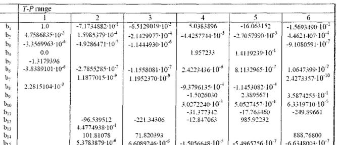
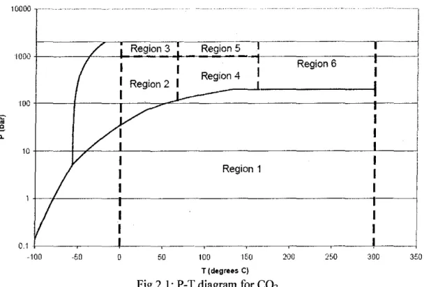
where T and Pare in Kelvin and bar respectively. It becomes more complex as the P-T diagram of C02 is divided into six (6) sections, as such there 6 different sets of parameters to be fitted in.
In addition, there are 15 parameter coefficients needed to be fitted in the EOS in order to find any ljlc02 value. Below are shown the table of parameter coefficients as well as P-T diagram for COz.
T-Prange
I 1 3 4 5 6
b, 1.0 -7.1734SS2·1 o-r -6.5129019·10- 5.0383896 -16.06315" ·1.5693490· 10
b, 4.7586835·1Cr3 1.598.5379·10~ -2J4299i7·1
o·
4 -4.4~577--W·I0-3 -2.7057990 ·w·'
-1.4621407· 10"4 b3 -3.3569963·10'6 -4.9286471·10·-
-1.14H9.lo·w·'
-9.1080591·10'7b_. 0.0 1.957133 1.4119239·10'1
b5 -1.3179396
h;; -3.S38910I·l0·6 -2. 7855285·1 o·' -1.1558081· 10'7
2.4213436·10'6 8. 1132965 ·10' 7 1.06-P399·10-7
h~ 1.1877015·10"9 1.1952370·10·' 2A2i.BJ7-l o-Jo
b, 2.2815104·1Cf3 -9.3796135·10~ -1.1453082· JO"
h; -1.5026030 2.3895671 3.5874255·10'1
bw 3.02722-to-1 o·3 5.0527457·10'4 6.3319710·!0'5
bn -31._::773+2 -17.763460 -249.89661
bl~ -96539512 -2.:!.1.3-l-306 -12.84-7063 985.9.:!..:!.32
bu 4-..:l-i74938·10"1
bt~ 101.81078 71.820393 888.76800
bl5 5.3i83Si9·10-6 6.6089246·1
o·
6 -1.5056648· 10'5 -5.-1.965:!%·10"7 -6.6348003·10"7Table 2.1: Parameter coefficients for Eq. 2
1: 273 K<J'<573 K, P<P1 (when T<305 K, P, equals 1o the saturation pressure of C02 ; when 305 K<T<405 K,
P1~75+(T-305)-1.25; when 1'>405 K, P,~200 bar.); 2: 273 K<f<340 K, P1<1'<1000 bar; 3: 273 K<T<340 K, P
>1000 bar; 4:340 K<l'<435 K, P1<P<IOOO bar; 5:340 K<f<435 K, P>JOOO bar; and 6: T>435 K, P>P1•
10000
1000 Region 3
---!
~Qior1s' ---.,---]
~--~~~--~--~~
Region 6 : Region 4 I
Region 1
0.1 -f----~---1---~---~-~~-~--~- _ _
_,___----j
-100 -50 0 50 100 150 200 250 300 350
T (degrees C)
Fig 2.1: P-T diagram for C02
1: 273 K<f<573 K, P<P1 (when T<305 K, P1 equals to the saturation pressure of C02; when 305 K<f<405 K,
r,~75+(T-305)-1.25; when T>405 K, r,~2oo bar.); 2: 273 K<J'<340 K, P1<P<JOOO bar; 3: 273 K<r<340 K, P
>1000 bar; 4:340 K<f<435 K, P1<P<IOOO bar; 5:340 K<r<435 K, P>IOOO bar; and 6: T>435 K, P>P,,
Thus, this project intends to design a single model to calculate the value of <!>em for whole regions. However, since the relationship between fugacity, temperature, and pressure are expected highly non-linear, it is assumed that Neural Network (NN) is able to provide suitable solution for the project.
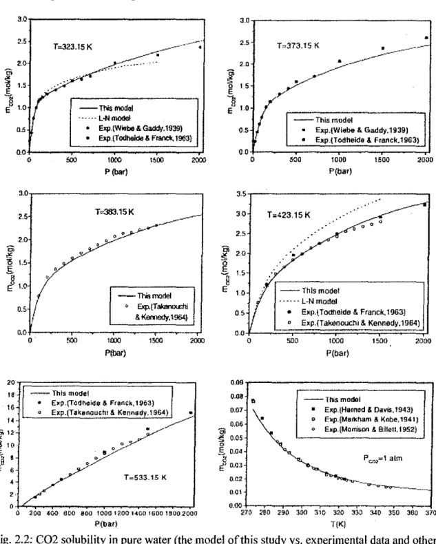
2.2.1. Comparison with Experimental Data
3.0.,..---,
.2.5
T=323.15 K ~ -~~--.·
r:: -~·-·· ~
; 10 r r=~::::::-ThiS--- .... -d.-~---.
--- --- L-N modo!
0.5 • E>ql.(W~bo&Ga<ldy.1939)
• E>ql(fodh<lldo6flllnel<, 1963)
o.oL--~::::::::::;::::::::::;:::::;:::=:,J
0 1000
P (bar)
1500
3 . 0 , - - - ,
2.5 T•383.15K ---
2.0
~
.~J--
~ ~
r: ,./ I
--llio mortel
o . .s ; ~ 5cp.t1~i
~~~--~-~~:;::=::&::K:Il0!1<0Cjy~=·1:96<=)
0.0~ --~
0 ro.1 1 IX() 1 sco 2000
P(bar)
••r,===========::::;---.
18 - - - Thts model
;r, • E)lp.(HdMidO & FtMCk, 1963)
<~ Exp.(Takenouchi & Kannady.1964) •
,.
~,1~ ~
~TO o/~y
1·
E :/_y//
T=533.15 K, .
•• ~~~-~---T-~~-~__) o 200 400 ac•o aoo tooo 1200 14oo tGOo tsoo2ooo
a;
3.0~---~
2.5
2.0
1 -o
1 5E
To373.15 K
. -- ---
•/---
(
--Thl:smodel
0.5 Exp.lWiebe & Gaddy,1'939)
• Exp.(Todheide & Fra.ntk.1963) } 10
0 0
L--..':::;:==:;::===:;:==!.1
0 500 1000
P(bar)
1500 2000
3.5-.--...;_ _ _ _ _ _ _ _ _ _ _ _ -,
30 2.5
(I Q 0 u
---L-Nmodal
• E)lp.(Toatl~lde & Fnmck,1963) o Exp.{TakOOoucl"'i & Kennedy,19fl4) 0 0
_ji_._.!:::::;:::::=.=:.=::::::;:===:,;=::::::.';:=::;J
0 500
0.09 0.08 0.07
•
0.06 •
1000 P(bar)
--This modo!
15.;)1}
• Exp.{Hatncd & Oavi!i, 1943}
2000
o Ellp.(M~;~Ikham & Kobe,1941) o E)Cp.{Morris.on & 8ille11, 1952)
~ 0.05
E. 0 0.04
Es o.a3 P r.:n~=1 alm
0.02
o.ot
P(Mrl T(K)
Fig. 2.2: C02 solubility in pure water (the model of this study vs. experimental data and other models)
Based on the figures above we can conclude that comparison with experimental data demonstrates that this model gives results within or close to experimental uncertainty (about 7%)
in the temperature range from 273 to 533 K, for pressures from 0 to 2000 bar. Following the approach adopted by Duan et al. (1992a); this model is extended to predict C02 solubility in more complex brines such as seawater with remarkable accuracy.
2.3. Neural Network
2.3.1. History Perspective
The field of artificial neural networks (they also go by the names of connectionist models, parallel distributed processing systems and neuromorphic systems) is very active nowadays.
Although for many people artificial neural networks can be considered a new area of research, which developed in the late eighties, work in this field can be traced back to more than fifty years ago. McCulloch and Pitts, back in 1943, pointed out the possibility of applying Boolean algebra to nerve net behaviour. They essentially originated neurophysiological automata theory and developed a theory of nets. In 1949 Donald Hebb, in his book "The organization of behavior'' postulated a plausible qualitative mechanism for learning at the cellular level in brains. An extension of his proposals is widely known nowadays as the Hebbian learning rule.
In 1957 Rosenblatt developed the first neurocomputer, the perceptmn. He proposed a learning rule for this first artificial neural network and proved that, given linearly separable classes, a perceptron would, in a finite number of training trials, develop a weight vector that would separate the classes (the famous Perceplron convergence theorem). His results were summarized in a very interesting book, "Principles of neurodynamics ".
About the same time Beman! Widrow modelled learning from the point of view of minimizing the mean-square error between the output of a different type of ANN processing element, the AD ALINE, and the desired output vector over the set of patterns. This work has led to modern adaptive filters. Adalines and the Widrow-Hoff'learning rule were applied to a large number of problems, probably the best known being the control of an inverted pendulum.
Although people like Bernard Widrow approached this field from an analytical point of view, most of the research on this field was done from an experimental point of view. In the sixties many sensational promises were made which were not fulfilled. This discredited the research on
artificial neural networks. About the same time Minsky and Papert began promoting the field of artificial intelligence at the expense of neural networks research. The death sentence to ANN was given in a book written by these researchers, Perceptrons, where it was mathematically proved that these neural networks were not able to compute certain essential computer predicates like the EXCLUSNE OR boolean function. Until the 80's, research on neural networks was almost null. Notable exceptions from this period are the works of Amari, Anderson, Fukushima, Grossberg and Kohonen.
Then in the middle 80's interest in artificial neural networks started to rise substantially, making NN one of the most active current areas of research. The work and charisma of John Hopfield has made a large contribution to the credibility ofNN. With the publication of the PDP books the field exploded. Although this persuasive and popular work made a very important contribution to the success of NN, other reasons can be identified for this recent renewal of interest:
One is the desire is to build a new breed of powerful computers, that can solve problems that are proving to be extremely difficult for current digital computers (algorithmically or rulebased inspired) and yet are easily done by humans in everyday life. Cognitive tasks like understanding spoken and written language, image processing, retrieving contextually appropriate information from memory, are all examples of such tasks.
Another is the benefit that neuroscience can obtain from NN research. New artificial neural network architectures are constantly being developed and new concepts and theories being proposed to explain the operation of these architectures. Many of these developments can be used by neuroscientists as new paradigms tor building functional concepts and models of elements of the brain.
Also the advances of VLSI technology in recent years, turned the possibility of implementing NN in hardware into a reality. Analog, digital and hybrid electronic implementations are available today, with commercial optical or electrooptical implementations being expected in the future.
The dramatic improvement in processing power observed in the last few years makes it possible to perform computationally intensive training tasks which would, with older technology, required an unatfordable time.
Research into ANNs has lead to several different architectures being proposed over the years. All of them try, to a greater or lesser extent, to exploit the available knowledge of the mechanisms of the human brain. Before describing the structure of artificial neural networks we should give a brief description of the structure of the archetypal neural network.
2.3.2. Project Perspective
In this project, Neural Network (NN) will be used to generate a mathematical model which is able to calculate cflco2 for the whole regions of P-T diagram for C02• Thus, MATLAB is preferable computational software to be used for the project. The NN represents a complex configuration consists of many simple processors (or 'neurones'), arranged in layers (input, hidden and output layer). The proper transformation of information is possible as a result of correctly prepared matrix of weights, numbers attributed for the all interneuron's connections. In the most frequently used feed-forward network, each neurone simply. sums up (properly amplified or weaken) signals from the all neurones of the previous layer and, after transformation received result by suitable activation function transmits it to all neurones of the next layer. In addition, the learning process is executed on the basis of input data sets and associated with output data sets. During the learning process (supervised learning) computer compares the values calculated with the expecting ones and adjusts step by step the weight's values to reach the best agreement between the six data sets. In the end of the computational activity, it is expected that a single model to calculate cfle02 is able to be generated by MA TLAB.
Finally, the model value of <!>em is compared with the experimental value <!>em in order to validate the model.
CHAPTER3
METHODOLOGY
3.1. Methodology
~
• To do literature review on C02-H20 fugacity & data collection.I
~
2 • To identify the parameters of fugacity coefficients calculation.I
~
3 • To reproduce the fugacity parameters.I
~
y
• To do literature review on neural network.J
~
5 • To program on how neural network can be used to calculate fugacity.]
~==·=To=:de:v:e:lo:p:a::n:eu:r:a:ln:e:t:w:o:rk::m:o:d:e:l.::::::=:=:::=:=:::=:=:::~)
/.7 • To validate the accuracy of designed model with original model.
3.2. Gantt Chart
No Activities
Fig 3.1: Gantt Chart of Project
CHAPTER4
RESUI,TS AND DISCUSSION
4.1. Results
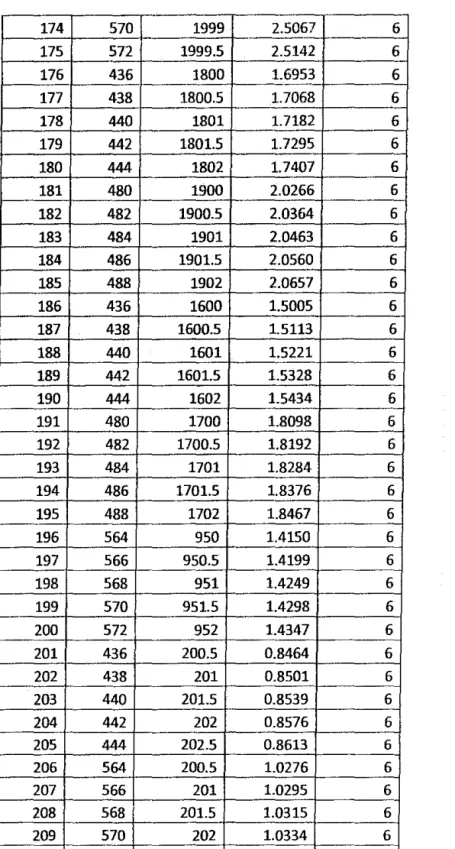
After collecting data of temperature, pressure as well as actual C02 fugacity coefficients, <(>co2
Actual. the neural network model has been designed based on try-and-error method. Besides, all data which used for simulation are randomly picked. However, the data are taken from the whole 6 regions in order to preserve the accuracy of the results at the end of the simulation. Recall that the formula used to get the outputs is equation (32) which is:
<!>co, = bt
+ [hz +
b3T+ ~ +
(T~~SO)]
P+
[b6+
b7T+ ~]
P2+
[b9+
b10T+ b~
1]tnP
+
[b12+
b13T]+
b14+
b T2p T ts
Thus, the actual outputs, <!>em Actual are fugacity coefficients of CO:l-l-120 system calculated based on formula above, while <!>em Sim are simulation outputs generated by neural network. Based on the table below, there is a "Region" column which represents the region ofP- T diagram for C02 (Fig I). Do take note that for region "I" of P-T diagram of C02, it has been divided into 3 parts due to conditions (P, T).
No T (K) P (bar) 4»coz Actual Region
1 274 1 0.9932 1 (Part 1)
2 276 1.5 0.9901 1 (Part 1)
3 278 2 0.9871 1 (Part 1)
4 280 2.5 0.9842 1 (Part 1)
5 282 3 0.9815 1 (Part 1)
6 284 3.5 0.9789 1 (Part 1)
7 286 4 0.9765 1 (Part 1)
8 288 4.5 0.9742 1 (Part 1)
9 290 5 0.9720 1 (Part 1)
10 292 5.5 0.9699 1 (Part 1)
11 294 6 0.9679 1 (Part 1)
12 296 6.5 0.9660 1 (Part 1)
13 298 7 0.9642 1 (Part 1)
14 300 7.5 0.9625 1 (Part 1)
15 302 8 0.9608 1 (Part 1)
16 545 143 0.9488 1 (Part 1)
17 547 143.5 0.9498 1 (Part 1)
18 549 144 0.9508 1 (Part 1)
19 551 144.5 0.9517 1 (Part 1)
20 553 145 0.9527 1 (Part 1)
21 555 145.5 0.9536 1 (Part 1)
22 557 146 0.9545 1 (Part 1)
23 559 146.5 0.9554 1 (Part 1)
24 561 147 0.9562 1 (Part 1)
25 563 147.5 0.9571 1 (Part 1)
26 565 148 0.9579 1 (Part 1)
27 567 148.5 0.9587 1 (Part 1)
28 569 149 0.9596 1 (Part 1)
29 571 149.5 0.9603 1 (Part 1) 30 572 150 0.9607 1 (Part 1)
31 306 76 0.6624 1 (Part 2)
32 308 76.5 0.6677 1 (Part 2)
33 310 77 0.6729 1 (Part 2)
34 312 77.5 0.6780 1 (Part 2)
35 314 78 0.6830 1 (Part 2)
36 316 78.5 0.6879 1 (Part 2)
37 318 79 0.6927 1 (Part 2)
38 320 79.5 0.6974 1 (Part 2)
39 322 80 0.7020 1 (Part 2)
40 324 80.5 0.7065 1 (Part 2)
41 326 81 0.7110 1 (Part 2)
42 328 81.5 0.7154 1 (Part 2)
43 330 82 0.7197 1 (Part 2)
44 332 82.5 0.7239 1 (Part 2)
45 396 170 0.7278 1 (Part 2)
46 398 170.5 0.7325 1 (Part 2)
47 400 171 0.7372 1 (Part 2)
48 402 171.5 0.7418 1 (Part 2)
49 404 172 0.7463 1 (Part 2)
50 406 150 0.7772 1 (Part 3)
51 408 150.5 0.7810 l(Part3)
52 410 151 0.7847 l(Part3)
53 412 151.5 0.7883 1 (Part 3)
54 414 152 0.7919 1 (Part 3}
55 416 152.5 0.7954 1 (Part 3)
56 418 153 0.7989 1 (Part 3)
57 420 153.5 0.8023 l(Part3)
58 422 154 0.8057 l(Part3)
59 424 154.5 0.8090 1 (Part 3) 60 564 197.5 0.9452 1 (Part 3)
61 566 198 0.9462 1 (Part 3}
62 568 198.5 0.9472 1 (Part 3)
63 570 199 0.9482 l(Part3)
64 572 199.5 0.9492 l(Part3)
65 274 900 0.1474 2
66 276 900.5 0.1527 2
67 278 901 0.1580 2
68 280 901.5 0.1635 2
69 282 902 0.1690 2
70 284 902.5 0.1747 2
71 286 903 0.1804 2
72 288 903.5 0.1862 2
73 290 904 0.1920 2
74 292 904.5 0.1980 2
75 331 997.5 0.3420 2
76 333 998 0.3497 2
77 335 998.5 0.3574 2
78 337 999 0.3652 2
79 339 999.5 0.3731 2
80 300 500 0.2071 2
81 302 500.5 0.2132 2
82 304 501 0.2193 2
83 306 501.5 0.2256 2
84 308 502 0.2319 2
85 274 200.5 0.1953 2
86 276 201 0.2025 2
87 278 201.5 0.2099 2
88 280 202 0.2173 2
89 282 202.5 0.2247 2
90 331 200.5 0.4411 2
91 333 201 0.4502 2
92 335 201.5 0.4592 2
93 337 202 0.4684 2
94 339 202.5 0.4775 2
95 331 1000.5 0.3416 3
96 333 1001 0.3493 3
97 335 1001.5 0.3570 3
98 337 1002 0.3648 3
99 339 1002.5 0.3727 3
100 274 1995 0.3725 3
101 276 1995.5 0.3830 3
102 278 1996 0.3936 3
103 280 1996.5 0.4043 3
104 282 1997 0.4150 3
105 284 1997.5 0.4259 3
106 286 1998 0.4368 3
107 288 1998.5 0.4479 3
108 290 1999 0.4590 3
109 292 1999.5 0.4702 3
110 330 1500 0.4641 3
111 332 1500.5 0.4736 3
112 334 1501 0.4833 3
113 336 1501.5 0.4930 3
114 338 1502 0.5028 3
115 341 900 0.3647 4
116 343 900.5 0.3719 4
117 345 901 0.3791 4
118 347 901.5 0.3863 4
119 349 902 0.3936 4
120 351 902.5 0.4009 4
121 353 903 0.4082 4
122 355 903.5 0.4156 4
123 357 904 0.4230 4
124 359 904.5 0.4304 4
125 426 997.5 0.7013 4
126 428 998 0.7088 4
127 430 998.5 0.7162 4
128 432 999 0.7236 4
129 434 999.5 0.7310 4
130 341 200.5 0.4929 4
131 343 201 0.5005 4
132 345 201.5 0.5081 4
133 347 202
-
0.5156 4134 349 202.5 0.5230 4
135 426 200.5 0.7650 4
136 428 201 0.7689 4
137 430 201.5 0.7727 4
138 432 202 0.7765 4
139 434 202.5 0.7801 4
140 416 1995 1.1779 5
141 418 1995.5 1.1886 5
142 420 1996 1.1993 5
143 422 1996.5 1.2100 5
144 424 1997 1.2206 5
145 426 1997.5 1.2312 5
146 428 1998 1.2417 5
147 430 1998.5 1.2523 5
148 432 1999 1.2627 5
149 434 1999.5 1.2732 5
150 341 1000.5 0.3796 5
151 343 1001 0.3875 5
152 345 1001.5 0.3955 5
153 347 1002 0.4034 5
154 349 1002.5 0.4113 5
155 341 1500 0.5169 5
156 343 1500.5 0.5267 5
157 345 1501 0.5365 5
158 347 1501.5 0.5463 5
159 349 1502 0.5560 5
160 523 1995 2.3264 6
161 525 1995.5 2.3351 6
162 527 1996 2.3438 6
163 529 1996.5 2.3524 6
164 531 1997 2.3609 6
165 533 1997.5 2.3694 6
166 535 1998 2.3778 6
167 537 1998.5 2.3862 6
168 539 1999 2.3945 6
169 541 1999.5 2.4027 6
170 562 1997 2.4764 6
171 564 1997.5 2.4840 6
172 566 1998 2.4916 6
173 568 1998.5 2.4992 6
174 570 1999 2.5067 6
175 572 1999.5 2.5142 6
176 436 1800 1.6953 6
177 438 1800.5 1.7068 6
178 440 1801 1.7182 6
179 442 1801.5 1.7295 6
180 444 1802 1.7407 6
181 480 1900 2.0266 6
182 482 1900.5 2.0364 6
183 484 1901 2.0463 6
184 486 1901.5 2.0560 6
185 488 1902 2.0657 6
186 436 1600 1.5005 6
187 438 1600.5 1.5113 6
188 440 1601 1.5221 6
189 442 1601.5 1.5328 6
190 444 1602 1.5434 6
191 480 1700 1.8098 6
192 482 1700.5 1.8192 6
193 484 1701 1.8284 6
194 486 1701.5 1.8376 6
195 488 1702 1.8467 6
196 564 950 1.4150 6
197 566 950.5 1.4199 6
198 568 951 1.4249 6
199 570 951.5 1.4298 6
200 572 952 1.4347 6
201 436 200.5 0.8464 6
202 438 201 0.8501 6
203 440 201.5 0.8539 6
204 442 202 0.8576 6
205 444 202.5 0.8613 6
206 564 200.5 1.0276 6
207 566 201 1.0295 6
208 568 201.5 1.0315 6
209 570 202 1.0334 6
210 572 202.5 1.0353 6
Table 4.1: Data collection consists oftemperature, pressure & fugacity coefficient
As mention before, the neural network is basically built based on try-and-error approach, in term of the number of neurons, layers as well as type of transfer functions. Below are shown several results of this project, which will be discussed in 'Discussion' section:
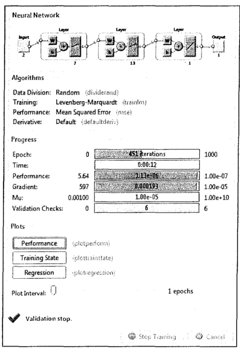
Neural Network
Algorithms:
Data Division: Random (di·iich::I-Mid_:
. Training: Levenberg-Marquardt (trainltr!}
Performance: Mean Squared Error i_m:ce:1 Derivative:
Progress
Epoch: 0
Time:
PErformance: 5.64 Gradient: 597 Mu: 0.00100 Validation Checks: 0 Plot>
'piG tJ·cg,· • .:::::ion!
Plot Interval: /] 1 epochs
~ Validation stop.
Fig 4.1: MA TLAB neural network
1000
l.OOe-07 l.OOe-05 1.00e+10 6
'-~-'11'1\:t:i
Best Validation Performance is 6.3027~ at epoch 445
--Train ---Validation ---Best ---Goal
--- -~---- _::::::_----:::::_--:?--- -=~--e
10-e
---1-
'
10~~--~----~--~----~--~----~--~----~--~
0 50 100 150 200 250 300 350 400 450
451 Epochs
Fig 4.2: Performance of neural network
8 q
2.5~ cP 2
"' -
+ Ill-
Q) 1 .5I-Ill
"
...-
1- '
:::JB-
0.5:::J
0
2.5
0)
...-
0 0 0 2
q
-
+& -
15I-Ill
..
...-'
1....
:::J
B-
0.5:::J
0
Training: R=1
0 Data - - F i t --- Y=T
0.5 1 1.5
Target
All: R=1
0 Data - - F i t --- Y=T
0.5 1 1.5
Target
2 2_5
2 2.5
Validation: R=0-99999
0 Data ---Fit 2 --- y
=
T'
....
:::J
B-
0.5:::J
0
0.5 1 1.5 2
Target
Fig 4.3: Regression plot of neural network
3 2.5 1:' ~
·o 2
~ 8 1.5
~
·'5
..
g' u.. 0.5
0 2000
... ··
.. _.···
.... ···
...
:
.... ···... ··
1500 1000
500 .. ··
... ··
Simulation .-··
.··
300
··.·-.
· ..
-~-
500
Pressure(bar) 0 200
Temperature(!<)
Fig 4.4: 30 plot ofP-T-rl>cozs1m
Warning: NEiiFF u!led J.n a.."l. cb.esalete wa:,.•.
> In ab!l u!le at 18
In neYif:f>create net1r10rk at 127 In ne'.olf:f at 102
In syafig6 at 26
See help for UEWFF to ·.:~pdatt: call!! to the new arg:.m.ent l i g t .
l)Weighc val:1e(.s) for hidden layer {IH):
ans =
0.024314886198726 0.027122406187101 0.103436929229812 0. 030422688264001 -0.060150865352321 0. 01El7;!4145'l435'lD -0.400073302631029
0. 009201900343075 -0.028571475158761 -0 • .13680"1.7':l1773623 -0.003984725995334 O.OE8319019057763 0. 00242325:1'135431 D.0913016903"1.2338
2)3ias value(s) for 1st hidden layer(31):
an!! =
-29.611673V19~B9301
-21.659270012541863
-17.2127~9648478820
-7.116523562434156 16.349496547615362 -10.565619290653!:-22 -8.219902175068270
Fig 4.5: Weights & biases for I'' hidden layer
600
.J..., •• , .... .;•, .·•,: .•. ·
"S)We:ight; value(!!!) terr 2nd h:idden layer(LWl):
a.2eo6i'H71695aao -3- 221516655521 0~ 9 -4 .54'J!I1'92U65757J i . 92SS95609273~i'.5 -1.502 92065500914·' -3.H23'>36UB21S3~
3.2972114BOSMSS 1.512321424nSS32 1.4570~9686'!336~6 -3-12.5285302265443 5.52'1129558-l. 74433 0.38166648001160~
l • .'l~06061801J~1120
-6.05725304542~375 9.00U565657~2~27 0.2H71013164890S -0.099713661 '142174 2 .Cd1072602020'172 3-622917990692167 3. 986B1142llES496 -3.784195501300252 -0.79Q09H~H1~D69
5.BOS1079521194'J
~ .01E7l022l49151CI -s. 390os 65 52 so~ 513 -0.061l1536B2217420
3. 599753676215316 1. 7097695().95~7£-9~
-0. 5905 61518121666 "-336708~5~99:;,165 0.241l>l740S1247H -li. 'J~9521i00999U~2 3.1101i'.13B964396S -2. 960413~25273762 1..373196377226'>52 -~.1.,J9o967rr49~J5 -3-~21!1563 66332 052 2 .16SE6S919516351 -~-63608559131?566 -2 .115~S96016Sn75
2. 65~320g60893S95 3. 72912140J9l129S 1.7118612588039iS -D. 35~ 712 D160 S 6593 -1.4161462058\16159 -5.086590135~5;253
~').117426919116182 4. 017~363737~92:20
-2 .8t4?8115'J162 306 -s. ~4566233625e<:>s -2.736134545609030 ' - se3o376tB.n2 '16s
~.1525~719%Se~ 8:; -5. 5~·-·~~::.s~:;, n 1so1 2. 5603~e515SB9~9 1 .o1 ~S56lel5s9n.) -L 9~31~9~ 53~0~!110 -3.75901US16H5~3 2. 43J.'>l56~354H99 0. 272S-Jl57 Bi'.li7•J1 3. 42il6JllS439110~
s. 'l~S:S1119132€923 -5. ~5~514-!.<5721900 -i.109SOO~S6S62563 5. ~0!55lS06185101 2. C•9~1:;,7lE9507l03 -3.4363710502215~7 -0.2'1~552103551318 s. s~~e166nS22179 -Q. n~B~06S66Sll58 1. 6EIS6~5:!51()Q7005 ~. ~9C6l2T!76l12l.'l -s.oHi9171=ss~~s7 -·J.06~~~99S6S2e7le ~. ~-JBl 032 557S51-l B.1321!1H59lt;S~2~
-1. 75~5692!7-B2~·6S -3. ~65g:52C•l11 H99 -2. 'l90625961-i23565 2.Utl25S~H'l35~5~2 1. 95S~865li6365~9B -4-6602'10'15400~'!80 -D. 06;92 90~52S,S252 1. 9JO 22507896150 -5. 79i305007l6"Z·J17
1.1605ei1UJOS06iO ~ .60l ;s~31a~6l61 9. 9•:.5072-!555H~.,6 -o. ~!15151519321ns -5.21'3 3Tl76~H017 7 .3SOl2S0525669lS
Fig 4.6: Weights & biases for 2"d hidden layer
Fig 4.7: Weights & biases for output neuron
-S.n66556UH2573 -5.5012 69159559M~
3.07n973B255l06S D.l692BS7Mrl1l15 5. H652630llS926i 1.17726724131£895 2 .1ses10'l5651S60s -0 6302l12959.'!31H 1. B21B0210000352l 2. ~205532li9215U5
--1. 167~Jc76555673e 0. 936724':l37l5Cill -6. ~B'J:i27~ e'/SUC.~ J.
= = = = = = = Hodel Testing seceion
Please enter- number of desired data = 3
Enter Iemperature(R) 1( 273K<Temperature<573K 300 Enter Temperature(K) 2( 273K<Ten::perature<573K 400 Enter Temperature (K) 3 ( 273K<T~-erature<573K 500 Enter Pre.ssure(bar) 1( 0<Pressure<2000bar 1000 Enter Pressure(bar) 2( 0<Pressure<2000bar 1500 Enter Pres5ure (bar} S ( 0<Pressu:re<2000bar 1999 Output 1 0.239254
Output 2 OUeput 3
A» I
1.0H668 2.247637
Fig 4.8: Model testing
No T (K) P (bar) «<»co2 Actual t!Jcozslm
1 274 1 0.9932 0.9930
2 276 1.5 0.9901 0.9902
3 278 2 0.9871 0.9873
4 280 2.5 0.9842 0.9844
5 282 3 0.9815 0.9816
6 284 3.5 0.9789 0.9789
7 286 4 0.9765 0.9763
8 288 4.5 0.9742 0.9739
9 290 5 0.9720 0.9717
10 292 5.5 0.9699 0.9697
11 294 6 0.9679 0.9678
12 296 6.5 0.9660 0.9660
13 298 7 0.9642 0.9643
14 300 7.5 0.9625 0.9626
15 302 8 0.9608 0.9608
16 545 143 0.9488 0.9469
17 547 143.5 0.9498 0.9488
18 549 144 0.9508 0.9505
Error(%) 0.0197 0.0123 0.0226 0.0183 0.0063 0.0076 0.0188 0.0243 0.0228 0.0151 0.0037 0.0078 0.0145 0.0112 0.0074 0.2083 0.1045 0.0337
Region 1 (Part 1) 1 (Part 1) 1 (Part 1) 1 (Part 1) 1 (Part 1) 1 (Part 1) 1 (Part 1) 1 (Part 1) 1 (Part 1) 1 (Part 1) 1 (Part 1) 1 (Part 1) 1 (Part 1) 1 (Pa'rt 1) 1 (Pa'rt 1) 1 (Pa:rt 1) 1 (Pa'rt 1) 1 (Pa'rt 1)
19 551 144.5 0.9517 0.9518 0.0093 1 (Part 1)
20 553 145 0.9527 0.9529 0.0297 1 (Part 1)
21 555 145.5 0.9536 0.9539 0.0331 1 (Part 1)
22 557 146 0.9545 0.9547 0.0247 1 (Part 1)
23 559 146.5 0.9554 0.9555 0.0099 1 (Part 1)
24 561 147 0.9562 0.9562 0.0066 1 (Part 1)
25 563 147.5 0.9571 0.9569 0.0204 1 (Part 1)
26 565 148 0.9579 0.9577 0.0278 1 (Part 1)
27 567 148.5 0.9587 0.9585 . 0.0255 1 (Part 1)
28 569 149 0.9596 0.9594 0.0114 1 (Part 1)
29 571 149.5 0.9603 0.9605 0.0163 1 (Part 1)
30 572 150 0.9607 0.9608 0.0103 1 (Part 1)
31 306 76 0.6624 0.6622 0.0383 1 (Part 2)
32 308 76.5 0.6677 0.6679 0.0256 1 (Part 2)
33 310 77 0.6729 0.6732 0.0510 1 (Part 2)
34 312 77.5 0.6780 0.6783 0.0499 1 (Part 2)
35 314 78 0.6830 0.6832 0.0320 1 (Part 2)
36 316 78.5 0.6879 0.6879 0.0054 1 (Part 2)
37 318 79 0.6927 0.6925 0.0230 1 (Part 2)
38 320 79.5 0.6974 0.6970 0.0476 1 (Part 2)
39 322 80 0.7020 0.7016 0.0636 1 (Part 2)
40 324 80.5 0.7065 0.7061 0.0671 1 (Part 2)
41 326 81 0.7110 0.7106 0.0548 1 (Part 2)
42 328 81.5 0.7154 0.7152 0.0241 1 (Part 2)
43 330 82 0.7197 0.7198 0.0274 1 (Part 2)
44 332 82.5 0.7239 0.7246 0.1016 1 (Part 2)
45 396 170 0.7278 0.7277 0.0036 1 (Part 2)
46 398 170.5 0.7325 0.7328 0.0401 1 (Part 2)
47 400 171 0.7372 0.7375 0.0492 1 (Part 2)
48 402 171.5 0.7418 0.7412 0.0764 1 (Part 2)
49 404 172 0.7463 0.7436 0.3544 1 (Part 2)
50 406 150 0.7772 0.7767 0.0685 1 (Part 3)
51 408 150.5 0.7810 0.7807 0.0275 1(Part3)
52 410 151 0.7847 0.7847 0.0003 1 (Part 3)
53 412 151.5 0.7883 0.7884 0.0154 1 (Part 3)
54 414 152 0.7919 0.7921 0.0213 1 (Part 3)
55 416 152.5 0.7954 0.7956 0.0189 1 (Part 3)
56 418 153 0.7989 0.7990 0.0093 1(Part3)
57 420 153.5 0.8023 0.8022 0.0069 1 (Part 3)
58 422 154 0.8057 0.8054 0.0291 1 (Part 3)
59 424 154.5 0.8090 0.8085 0.0571 1 (Part 3)
60 564 197.5 0.9452 0.9457 0.0549 1 (Part 3)
61 566 198 0.9462 0.9461 0.0171 1(Part3)
62 568 198.5 0.9472 0.9466 0.0635 1 (Part 3)
63 570 199 0.9482 0.9478 0.0482 1 (Part 3)
64 572 199.5 0.9492 0.9497 0.0593 1 (Part 3)
65 274 900 0.1474 0.1491 1.1811 2
66 276 900.5 0.1527 0.1538 0.7760 2
67 278 901 0.1580 0.1587 0.4275 2
68 280 901.5 0.1635 0.1637 0.1314 2
69 282 902 0.1690 0.1688 0.1166 2
70 284 902.5 0.1747 0.1741 0.3207 2
71 286 903 0.1804 0.1795 0.4846 2
72 288 903.5 0.1862 0.1850 0.6121 2
73 290 904 0.1920 0.1907 0.7069 2
74 292 904.5 0.1980 0.1964 0.7725 2
75 331 997.5 0.3420 0.3437 0.4939 2
76 333 998 0.3497 0.3509 0.3580 2
77 335 998.5 0.3574 0.3582 0.2157 2
78 337 999 0.3652 0.3655 0.0676 2
79 339 999.5 0.3731 0.3728 0.0856 2
80 300 500 0.2071 0.2079 0.4095 2
81 302 500.5 0.2132 0.2137 0.2410 2
82 304 501 0.2193 0.2196 0.1074 2
83 306 501.5 0.2256 0.2256 0.0095 2
84 308 502 0.2319 0.2317 0.0519 2
85 274 200.5 0.1953 0.1974 1.0994 2
86 276 201 0.2025 0.2030 0.2442 2
87 278 201.5 0.2099 0.2088 0.4918 2
88 280 202 0.2173 0.2148 1.1151 2
89 282 202.5 0.2247 0.2211 1.6320 2
90 331 200.5 0.4411 0.4417 0.1345 2
91 333 201 0.4502 0.4514 0.2661 2
92 335 201.5 0.4592 0.4609 0.3586 2
93 337 202 0.4684 0.4703 0.4109 2
94 339 202.5 0.4775 0.4795 0.4221 2
95 331 1000.5 0.3416 0.3443 0.7907 3
96 333 1001 0.3493 0.3515 0.6428 3
97 335 1001.5 0.3570 0.3588 0.4881 3
98 337 1002 0.3648 0.3660 0.3272 3
99 339 1002.5 0.3727 0.3733 0.1611 3
100 274 1995 0.3725 0.3731 0.1651 3
101 276 1995.5 0.3830 0.3832 0.0645 3
102 278 1996 0.3936 0.3935 0.0148 3
103 280 1996.5 0.4043 0.4040 0.0704 3
104 282 1997 0.4150 0.4146 0.1004 3
105 284 1997.5 0.4259 0.4255 0.1037 3
106 286 1998 0.4368 0.4365 0.0796 3
107 288 1998.5 0.4479 0.4477 0.0280 3
108 290 1999 0.4590 0.4592 0.0504 3
109 292 1999.5 0.4702 0.4709 0.1549 3
110 330 1500 0.4641 0.4641 0.0057 3
111 332 1500.5 0.4736 0.4738 0.0367 3
112 334 1501 0.4833 0.4833 0.0118 3
113 336 1501.5 0.4930 0.4927 0.0524 3
114 338 1502 0.5028 0.5022 0.1200 3
115 341 900 0.3647 0.3624 0.6247 4
116 343 900.5 0.3719 0.3700 0.5113 4
117 345 901 0.3791 0.3775 0.4022 4
118 347 901.5 0.3863 0.3852 0.2957 4
119 349 902 0.3936 0.3928 0.1902 4
120 351 902.5 0.4009 0.4006 0.0842 4
121 353 903 0.4082 0.4083 0.0240 4
122 355 903.5 0.4156 0.4161 0.1355 4
123 357 904 0.4230 0.4240 0.2515 4
124 359 904.5 0.4304 0.4320 0.3728 4
125 426 997.5 0.7013 0.7011 0.0382 4
126 428 998 0.7088 0.7084 0.0491 4
127 430 998.5 0.7162 0.7159 0.0378 4
128 432 999 0.7236 0.7236 0.0010 4
129 434 999.5 0.7310 0.7314 0.0643 4
130 341 200.5 0.4929 0.4898 0.6261 4
131 343 201 0.5005 0.4987 0.3611 4
132 345 201.5 0.5081 0.5075 0.1246 4
133 347 202 0.5156 0.5160 0.0831 4
134 349 202.5 0.5230 0.5244 0.2619 4
135 426 200.5 0.7650 0.7678 0.3596 4
136 428 201 0.7689 0.7673 0.2095 4
137 430 201.5 0.7727 0.7689 0.4907 4
138 432 202 0.7765 0.7741 0.3044 4
139 434 202.5 0.7801 0.7839 0.4886 4
140 416 1995 1.1779 1.1778 0.0077 5
141 418 1995.5 1.1886 1.1885 0.0080 5
142 420 1996 1.1993 1.1993 0.0032 5
143 422 1996.5 1.2100 1.2100 0.0024 5
144 424 1997 1.2206 1.2206 0.0043 5
145 426 1997.5 1.2312 1.2312 0.0005 5
146 428 1998 1.2417 1.2417 0.0018 5
147 430 1998.5 1.2523 1.2524 0.0116 5
148 432 1999 1.2627 1.2628 0.0004 5
149 434 1999.5 1.2732 1.2732 0.0003 5
150 341 1000.5 0.3796 0.3802 0.1592 5
151 343 1001 0.3875 0.3875 0.0020 5
152 345 1001.5 0.3955 0.3949 0.1434 5
153 347 1002 0.4034 0.4023 0.2654 5
154 349 1002.5 0.4113 0.4098 0.3684 5
155 341 1500 0.5169 0.5153 0.3026 5
156 343 1500.5 0.5267 0.5254 0.2628 5
157 345 1501 0.5365 0.5358 0.1420 5
158 347 1501.5 0.5463 0.5466 0.0625 5
159 349 1502 0.5560 0.5580 0.3519 5
160 523 1995 2.3264 2.3266 0.0092 6
161 525 1995.5 2.3351 2.3352 0.0058 6
162 527 1996 2.3438 2.3438 0.0021 6
163 529 1996.5 2.3524 2.3523 0.0011 6
164 531 1997 2.3609 2.3608 0.0032 6
165 533 1997.5 2.3694 2.3693 0.0041 6
166 535 1998 2.3778 2.3777 0.0032 6
167 537 1998.5 2.3862 2.3862 0.0008 6
168 539 1999 2.3945 2.3946 0.0034 6
169 541 1999.5 2.4027 2.4030 0.0090 6
170 562 1997 2.4764 2.4763 0.0035 6
171 564 1997.5 2.4840 2.4842 0.0050 6
172 566 1998 2.4916 2.4919 0.0089 6
173 568 1998.5 2.4992 2.4994 0.0079 6
174 570 1999 2.5067 2.5068 0.0018 6
175 572 1999.5 2.5142 2.5139 0.0098 6
176 436 1800 1.6953 1.6943 0.0570 6
177 438 1800.5 1.7068 1.7068 0.0019 6
178 440 1801 1.7182 1.7193 0.0640 6
179 442 1801.5 1.7295 1.7317 0.1306 6
180 444 1802 1.7407 1.7442 0.2030 6
181 480 1900 2.0266 2.0263 0.0113 6
182 482 1900.5 2.0364 2.0365 0.0030 6
183 484 1901 2.0463 2.0465 0.0107 6
184 486 1901.5 2.0560 2.0563 0.0118 6
185 488 1902 2.0657 2.0658 0.0062 6
186 436 1600 1.5005 1.4983 0.1429 6
187 438 1600.5 1.5113 1.5113 0.0049 6
188 440 1601 1.5221 1.5236 0.0958 6
189 442 1601.5 1.5328 1.5353 0.1613 6
190 444 1602 1.5434 1.5464 0.1936 6
191 480 1700 1.8098 1.8091 0.0427 6
192 482 1700.5 1.8192 1.8185 0.0353 6
193 484 1701 1.8284 1.8281 0.0168 6
194 486 1701.5 1.8376 1.8378 0.0134 6
195 488 1702 1.8467 1.8477 0.0562 6
196 564 950 1.4150 1.4147 0.0181 6
197 566 950.5 1.4199 1.4201 0.0098 6
198 568 951 1.4249 1.4252 0.0226 6
199 570 951.5 1.4298 1.4301 0.0210 6
. 200 572 952 1.4347 1.4347 0.0061 6
201 436 200.5 0.8464 0.8294 2.0028 6
202 438 201 0.8501 0.8453 0.5660 6
203 440 201.5 0.8539 0.8563 0.2860 6
204 442 202 0.8576 0.8609 0.3866 6
205 444 202.5 0.8613 0.8591 0.2498 6
206 564 200.5 1.0276 1.0253 0.2285 6
207 566 201 1.0295 1.0293 0.0263 6
208 568 201.5 1.0315 1.0320 0.0553 6
209 570 202 1.0334 1.0339 0.0460 6
210 572 202.5 1.0353 1.0351 0.0206 6
Table 4.2: Genenc fugac1ty coefficients & errors
4.2. Discussion
After several tries, a quite precise neural network (NN)