A El Herbawi and Mr Borkhan B Jaafar for being supportive and guide me through

Stochastic Programming with Economic and Operational Risk Management in Petroleum Refinery Planning under Uncertainty

by

Nguyen Thi Huynh Nga

Dissertation submitted in partial fulfilment of the requirements for the

Bachelor of Engineering (Hons) (Chemical Engineering)

JANUARY 2009

Universiti Teknologi PETRONAS

Bandar Seri Iskandar 31750 Tronoh

Perak Darul Ridzuan

CERTIFICATION OF APPROVAL

Stochastic Programming with Economic and Operational Risk Management in Petroleum Refinery Planning under Uncertainty

by

Nguyen Thi Huynh Nga

A project dissertation submitted to the Chemical Engineering Programme Universiti Teknologi PETRONAS in partial fulfilment of the requirement for the

BACHELOR OF ENGINEERING (Hons) (CHEMICAL ENGINEERING)

Approved by,

(Cheng-Sebrfg Khor)

UNIVERSITI TEKNOLOGI PETRONAS TRONOH, PERAK

January 2009

CERTIFICATION OF ORIGINALITY

This is to certify that I am responsible for the work submitted in this project, that the original work is my own except as specified in the references and acknowledgements, and that the original work contained herein have not been undertaken or done by unspecified sources or persons.

A s

NGUYEN THI HUYNH NGA

ABSTRACT

Rising crude oil price and global energy concerns have revived great interests in the oil and gas industry, including the optimization of oil refinery operations. However, the economic environment of the refining industry is typically one of low margins with intense competition. This state of the industry calls for a continuous improvement in operating efficiency by reducing costs through engineering strategies. These strategies are derived based on an understanding of the world energy market and business processes, with the incorporation of advanced financial modeling and computational tools. Regard to the matter, this work proposes the application of the two-stage stochastic programming approach with fixed recourse to effectively account for both economic and operational risk management in the planning of oil refineries under uncertainty. The scenario planning and analysis approach is adopted to consider uncertainty in three parameters: prices of crude oil and commercial products, market demand for products, and production yields.

However, a large number of scenarios are required to capture the probabilistic nature of the problem. Therefore, to circumvent the problem posed by the resulting large- scale model, a Monte Carlo simulation approach is implemented based on the sample average approximation (SAA) technique. The SAA technique enables the determination of the minimum number of scenarios required yet still able to compute the true optimal solution of the problem for a desired level of accuracy within the specified confidence intervals. Two measures of risk are considered, namely mean-absolute deviation (MAD) and Conditional Value-at-Risk (CVaR). A representative numerical example is presented to illustrate the proposed modeling approach using GAMS modeling language with the nonlinear solver CONOPT3.

i n

ACKNOWLEDGEMENT

First and foremost, I would like to express my gratitude to my parents for giving me healthy life in this world. Thanks to my beloved and respected parents, I have been able do and accomplish so many things. And now I am here, having chance to research, understand and sail through all the difficulties to finish my final year project.

Secondly, a token of appreciation is for Mr Khor Cheng Seong, final year

project supervisor for his kind, enthusiastic guidance and advice throughout the progress of researching, developing model. In fact, Mr Khor has always helped me whenever I have problems from beginning until project's completion.

Deepest gratitude to the examiners for the seminars, and oral presentation Prof. Dr. Duwuri Subbarao , Ir. Dr. Abd Halim, Dr Murni Melati, Dr Mohanad M A

A El Herbawi and Mr Borkhan B Jaafar for being supportive and guide me through

the mistakes to make the project better. Thank you also to all lecturers and staffs that directly and indirectly involvedin making this project.

Moreover, I'd like to sincerely thank you to Final Year Project coordinator

for excellence guidance in organizing and constructing the seminar, oral

presentation.

Last but not least, special thanks to our family and colleagues for their support FYP something to be proud of. Thank you to all of you.

IV

ABBREVIATIONS AND NOMENCLATURES

Sets and Indices

/ set of materials/product i

IP set of materials/product i with price uncertainty

ID set of materials/product i with demand uncertainty

IY set of materials/product i with yield uncertainty

S set of scenarios s

K set of demand shortfall k\ and demand surplus kj

M set of yield shortfall m\ and yield surplus m%

N set of minimum number of scenario s

Parameters

C$,i unit price of raw materials and saleable products / with price uncertainty for

scenario s

Ps probability of each scenario s

di}k demand penalty for material i with demand uncertainty for either demand shortfall or surplus k

9i,m yield penalty for product i with yield uncertainty for either yield shortfall or surplus m

& weight factor, 6j, 62

a confident level

Continuous Variables

X material and saleable products flowrate

CVaR conditional- value- at- risk MAD mean absolute deviation

Zi.s.k demand penalty for material i in scenario 5 with demand uncertainty for either demand shortfall or surplus k

yi,s,m yield penalty for product i in scenario s with yield uncertainty for either yield shortfall or surplus m

Zo deterministic profit

$ monetary value of demand and yield penalty

M expected deterministic profit (x(z0) and expected demand and yield penalty

H confident interval

S(n) sampling variance estimator

z confident interval

Non-convex variables

VaR value-at-risk

v i

TABLE OF CONTENTS CERTIFICATION OF APPROVAL .

CERTIFICATION OF ORIGINALITY

ABSTRACT.

ACKNOWLEDGEMENT

ABBREVIATIONS AND NOMENCLATURES

CHAPTER 1:

CHAPTER 2:

CHAPTER 3:

CHAPTER 4:

INTRODUCTION .

1. Background of Study

2. Problem Statement

3. Objectives 4. Scope of study

THEORY 1.

2.

3.

4.

5.

6.

7.

9.

General formula of two-stage stochastic programming.

Two-Stage Stochastic Programming with Simple Recourse Subproblem Two-Stage Stochastic Programming

with Fixed Recourse Subproblem Two-Stage Stochastic Programming with Complete Recourse Subproblem.

Concepts from financial mathematics on risk measurement and risk management

Economic Risk

Value-at-risk (VaR) and Conditional-value-at-risk (CVaR)

Monte Carlo simulation approach

based on Sample Average Approximation .

Process flow network . . . .

METHODOLOGY 1.

2.

3.

4.

Optimization problem.

Monte Carlo simulation approach based on Sample Average Approximation (SAA) . General formulation of stochastic refinery planning with risk expressed in terms of MAD.

General formulation of stochastic refinery planning with risk expressed in terms of CVaR

RESULTS AND DISCUSSION 1. Numerical results 2. Discussion

li

i n

IV

10 11

13 13

14

16

17

19 19 27

CHAPTER5:

RERERENCES

APPENDICES

LIST OF FIGURES

Figure 1 VaR and CVaR illustration Figure 2 Process flow network

Figure 3 Cumulative distribution functions versus deterministic profit Figure 4 Cumulative distribution functions versus Penalty of demand and

yield

CONCLUSION AND RECOMMENDATION

1. Conclusion . . . .

2. Recommendation

29 29 30

31

33

9 11 23

25

LIST OF TABLES

Table 1 Period, nature of risk & risk metric 8 Table 2 Material balance around the units in the process flow network 11 Table 3 Lowerbound and upperbound of all material and products flow rate 14 Table 4 Flowrates of crude oil and saleable products 19

Table 5 Summary of computational result 19

Table 6 Deterministic profit and cumulative distribution function 21 Table 7 Penalty of yield and demand and cumulative distribution function 24

Table 8 (Values of) parameters 26

Table 9 Computational results 26

Table 10 Computational statistics of GAMS implementation for determining optimal solutions of MAD- and CVaR-based mean-risk stochastic

program 26

Table 11 Model statistics 27

Table 12 Model performance 27

Table 13 Comparison between MAD and CVaR 27

CHAPTER 1

INTRODUCTION

1. BACKGROUND OF STUDY

Stochastic Programming (SP) is a framework for modeling optimization that involves uncertainty. The following example of linear program helps to explain the concept of Stochastic:

in {ciXl +C2X2 +.... +CnXn] "\

m m

Subject to

aux\ + anxi +.... + ainXn < bi anxi + anx2+ .... + aznXn <bi

dm\X\ + (XmlX2 + .... + ClmnXn <. bn

X),X2,...,Xn >0

(1)

By using matrix vector notation, formulation (1) can be written as:

min cTx

s.t Ax < b

V

(2)

x>0 J

If b is a constant, the model is called Deterministic model. However, with b is uncertain, it is called Stochastic Model.

Two-stage Stochastic Programming with fixed recourse via scenario analysis is applied in Chemical process industry, oil and gas industry, water reservoir system, environment protection and control, etc... to predict planning under uncertainties and operational risk management by applying the concept of Variance, Mean Absolute Deviation (MAD) and Conditional-value-at-risk (CVaR)

Recourse is corrective action made after a random event has taken place. An example of two-stages Recourse is described as:

• Variables x: control the flow rate of Methane enters reactor to form Methanol.

• Random event: The control valve is malfunctioned and fully opened which results in the abundant amount of Methane fed into reactor, affecting the product quality.

• Recourse action y: To correct what has been messed up by the random event:

fix the control valve, penalty for overproduction of Methanol.

The above example includes two stages: the data for the first stage (x) are known with certainty and some data for the second stage are stochastic or random which need corrective action. Two-stage Stochastic Programming aims to serve the optimization purpose of a process by minimizing uncertainties and maximizing profit.

2. PROBLEM STATEMENT

The midterm refinery production planning problem addressed in this paper can be stated as follows. Given the following information:

• The available process units and their capacities;

• Cost of crude oil and refinery products;

• Market demand of products

Our goal is to determine our goal is to determine the amount of materials that are processed in each process stream of each process unit by considering the following uncertain parameters whose stochastic data (including probabilities) are available or

obtainable:

• Market demand for products, that is, production amounts of desired products;

Prices of crude oil and the saleable products; and

Product (or production) yields of crude oil from chemical reactions in the

crude distillation unit

•

It is assumed that:

• The uncertain parameters of prices, costs, and demands are externally imposed, that is, they are exogenous uncertainties;

• Further, the uncertain parameters are random variables that exhibit the behavior and properties of discrete probability distribution functions; and

• The physical resources of the plant are fixed.

3. OBJECTIVES

Following are the objectives of the project:

• There are large numbers of scenarios that create difficulty to handle various circumstances. For example, there may be more than thousands of cases happening. It is hard to predict and control numerous scenarios. Therefore, it is necessary to find the minimum number of scenarios to capture all the circumstances. Monte Carlo simulation approach based on the sample average approximation (SAA) technique is applied in this thesis to generate the minimum number of scenarios which present for thousands cases.

• The risk terms in Khor (2007) are handled using the metric mean-absolute deviation. After obtaining the first model with MAD as risk measurement, the second model is developed in which the risk terms are performed by CVaR. A comparison between the two models to assess which of these two risk measures is superior, both computationally and conceptually, in capturing the economic and operating risk in the planning of a refinery. Khor model (2007) is expressed:

mzKz^EizJ-eyizJ-E.-e.W (3)

where:

E[zo ]: Expected deterministic profit (crude oil and saleable products)

0,, #5 e (0, 1]: weight the components of the objective function V{z0): Variance of price uncertainty

E ,: Expected penalty of demand and yield uncertainties

W: MAD of demand and yield penalty

Apply MAD as risk measure:

max z=E[z0]-^MAD^ -E[^]-Q3MADZq (4)

Apply CVaR as risk measure:

max z=E[z0]~Q}CVaRi-E[Q-Q3CVaR): (5)

Solving optimization problem to find the input flow rate raw materials and final product to maximize profit.

4. SCOPE OF STUDY

• Monte Carlo simulation approach based on Sample Average Approximation (SAA) to determine minimum number of scenario

• General formulation of stochastic refinery planning with risk measure expressed in terms of MAD

• General formulation of stochastic refinery planning with risk measure

expressed in terms of CVaR.

CHAPTER 2 THEORY

1. GENERAL FORMULA OF TWO-STAGE-STOCHASTIC PROGRAMMING

The classical two-stage stochastic linear program (SLP) was originally proposed in the seminal works of Dantzig (1955) and Beale (1955) has the following general

form:

min cTx +EAQ(x,£(gj))1

s.t to Ax = b (6)

x e X > 0

where Q(x£((a)) =mm q1(g>)v

s.t. to W((d)y = h((o) - T((q)x (7)

v>0 With the notation:

x e Rn : Vector of first-stage decision variables, size (1x n) c : First-stage column vector of cost coefficient, sizes (n x 1) A : First-stage coefficient matrix, size (m x n)

b : Corresponding right-hand side vectors, size (m x 1)

(a e Q : Random events or scenario

£(co) : Random vector

q(ay) : Second stage vector of recourse cost coefficient vectors size (*xl)

A(co) : Second stage right-hand side vectors, size (/ x 1) T(($) : Matrix that ties the two stages together, size (/ x k) W(to) : Random recourse coefficient matrix, size (/ x k) y : Vector of second-stage decision variables, size (kx 1)

cTx is known as the first stage or "here and now" decision, x does not response to co. In contrast, y presents second stage variable with Q[x,^(g))) is "wait and see"

and is determined after observation regarding co has been obtained. Model (4) is the second stage problem, the recourse subproblem.

2. TWO-STAGE-STOCHASTIC PROGRAMMING WITH SIMPLE RECOURSE SUBPROBLEM

Simple recourse model is a special case of recourse model when recourse coefficients in the second stage, W, form an identity matrix. In general, we have:

e(*.«©))= £&(*,«©))

iel

Where:

Qi (x3 £(co)) =min q+uiy+i +q^y";

s.t. I y+i -1 y"i = A(©i) - (T'(co)x)/ (8)

y+i, y'i a)

h((x))-T(G>)x, a feasible solution to (5) is easily determined by setting y+ and y"

accordingly. Moreover, if the i* component of q+u - q^ >0, this feasible solution is

optimal.

Example of simple recourse is that when a target profit in one company is determined, the company will try to reduce the deviation from profit.

3. TWO-STAGE STOCHASTIC PROGRAMMING WITH FIXED RECOURSE SUBPROBLEM

Fixed recourse model is the model that the constraint matrix in the recourse

subprolem is fixed (not subject to uncertainty). (8) is written as:

Q(x£((q)) =min qT(®)y

s.t. Wy = h((o)-T(m)x (9)

y>0

When second stage objective coefficients are also fixed, the recourse subproblem

can be written as:

6(*,£(®))= min 7rT(A(co)-r(co)x) (10)

s.t. / W<qJ

7T=£)

4. TWO-STAGE STOCHASTIC PROGRAMMING WITH COMPLETE RECOURSE SUBPROBLEM

Aproblem is said to have complete recourse if Y(co, %) ={y \Way >x} is nonempty for any value of /and the recourse function is necessary finite, £>(x,£(co))=co.

Moreover, relatively complete recourse results if Y(a>,x)is nonempty for

all %e {h(co)-T(a))x \(a),x)eQxX'\.

With the complete recourse problem, model (4) becomes:

0(jc,4(<d)) =Min /(co)v +MeT z

s.tWy + z>h(a))~T(o))x, y,z>0 (11)

With M: large constant and e: appropriately dimensioned vector of ones.

5. CONCEPTS FROM FINANCIAL MATHEMATICS ON RISK

MEASUREMENT AND RISK MANAGEMENT

Three broad classes of risks are currently receiving wide attention and heavily studied in the literature related to financial mathematics, risk measurement, and risk management. The first, market risk, attempts to determine the uncertainty in the prices of an object that is traded in a liquid market. The second, credit risk, attempts

7

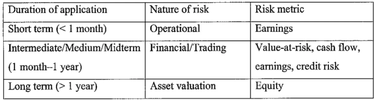
to place a value on the uncertainty associated with an account receivable. For example, researchers are interested in answering the question of how should we account for the possibility that a debtor may default on an obligation. The third, operational risk, basically tries to handle everything else. It considers the full set of other risks that a business must typically face, including the risk of catastrophic political events, weather-related risk, and risk of criminal activity (Pulleyblank, 2000). Table 1 provides examples of risk metrics or measures according to the duration of application and nature of risk involved.

Table 1: Period, nature of risk and risk metric Duration of application Nature of risk Risk metric

Short term (< 1 month) Operational Earnings

Intermediate/Medium/Midterm

(1 month-1 year)

Financial/Trading Value-at-risk, cash flow, earnings, credit risk Long term (> 1 year) Asset valuation Equity

6. ECONOMIC RISK

Economic risk is perceived by business people in two ways. The first is risk of not achieving the targeted financial objective. The second is the risk of variation in the results (Park and Sharp-Bette, 1990). The first type of risk may be caused by a number of causes whether economic, political, technical, or the like (of it), and can be represented as the probability of not achieving the financial objective. This type of risk has been employed with planning activities by Barbara and Bagajewicz (2003). The second type of risk can be well-handled by variance techniques such as the variance of Expected Monetary Value (EMV) (Bush and Johnson, 1998) or risk- adjusted return family of methods such as Sharpe ratio (Jones, 1998). Applequist et al. (2000) has adopted a risk premium defined as an increase in the expected return in exchange for a given amount of variance in order to evaluate risk and uncertainty for chemical manufacturing plants (Al-Sharrah, 2006).

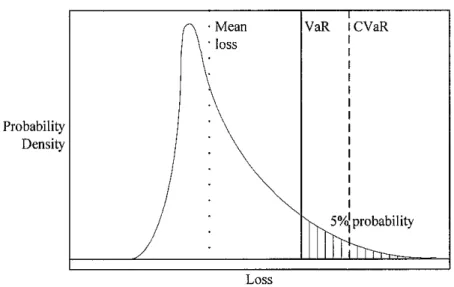
7. VALUE-AT-RISK (VAR) AND CONDITIONAL-VALUE-AT-RISK (CVAR)

Figure 1 expresses the idea about VaR and CVaR.

Probability Density

Loss

Figure 1: VaR and CVaR illustration

According to Rockafellar and Uryasev (2002), Value-atRisk (VaR) can informally be defined as a maximum loss in a specified period with some confidence level, except a (e.g., confidence level = 95%, period = 1 week). Formally, a -VaR is the a- percentile of the loss distribution. a-VaR is a smallest value such that probability that loss exceeds or equals to this value is bigger or equals to a. It suffers, however, from being unstable and difficult to work with numerically when losses are not normally distributed.

CVaR (Mean Excess Loss, Mean Shortfall or Tail VaR) is a risk assessment technique used to reduce the probability a portfolio will incur high losses. CVaR is performed by taking the likelihood (at a specific confidence level, example, 0.95 or 0.99, etc...) that a specific loss will exceed the value at risk (VaR). In mathematical point of view, CVaR is derived by taking a weighted average between the VaR and losses exceeding the VaR. CVaR maintains consistency with VaR by yielding the same results in limited settings where VaR computations are tractable, i.e., for

normal distribution. Most importantly for applications, CVaR can be expressed by a remarkable minimization formula. This formula can readily be incorporated into problems of optimization with respect to the decision vector x e Xthat are designed to minimize risk or shape in within the bounds. Significant shortcuts are thereby achieved while preserving crucial problem features like convexity.

8. MONTE CARLO SIMULATION APPROACH BASED ON SAMPLE

AVERAGE APPROXIMATION (SAA)

Two first step of SAA algorithm/steps proposed by Santoso et al. (2005):

Stepl: Generate M independent samples each of size N. For each sample solve the corresponding SAA problem

min^jcV^teO^/)} (12)

Step 2: Compute minimum number of scenario

Step 3: Apply risk measure into the model

(Referred to chapter 3 for more detail about the mathematical equation)

10

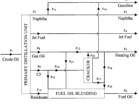
9. PROCESS FLOW NETWORK

Crude Oil Z

g

<

H

Q

>-

x7 -i *n

Naphtha

Jet Fuel

*8

Gas Oil

CF

Xi4

*15

*12

v*13

> ^20

u u

J. *I6

' l *18

u JC,7

1 ' X\s -^10

Residuum

FUEL OIL BLENDING

x2

Gasoline

*3

Naphtha

X4 Jet Fuel

JCs

Heating Oil

x6 Fuel Oil

Figure 2: Process flow network

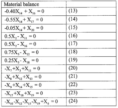
Table 2: Material balance around the units in the process flow network

Material balance

-0.40X14+X16=0 ⁽¹³⁾

-0.55X14+X]7 -0 (14)

-0.05XI4+X20=0 ⁽¹⁵⁾

0.5X2-Xn =0 ⁽¹⁶⁾

0.5X2-X16=0 ⁽¹⁷⁾

0.75X5-X12=0 ⁽¹⁸⁾

0.25X5-X18 =0 ⁽¹⁹⁾

-X7+X3+Xn =0 ⁽²⁰⁾

-X8+X12+X!3=0 (21)

-X9+X14+X15=0 ⁽²²⁾

-X17+Xl8+X]9 =0 (23)

-X10-X13-X15-Xl9+X5 =0 (24)

Materials and saleable products are divided into three groups

• Demand uncertainty (Xjd): X2, X3, X4, X5, X6

11

• Yield uncertainty (X\y): X4, X7, Xg, X9, Xio

• Price uncertainty (XiP): Xi, X2, X3, X4, X5, Xe, X(4

12

CHAPTER 3

METHODOLOGY

1. OPTIMIZATION PROBLEM

a) Objective

MAD: max z =E[zQ] -^MAD^ -E[^]-Q3MADZq, or CVaR : max z = E[z0] - QfiVaR^ ~E[Q - Q3CVaR^

b) Variables

• X;: material and saleable products

• Objective value: z ($/day)

• Penalty demand: Z(ID, S,K)

• Penalty yield: Y(IY,S, M)

c) Constrained equations of the model

X,< 15,000 (25)

X14<2,500 (26)

-Yield(S,IY)xX1+XIY+Y(IY,S,,Ml,)-Y(iY,S,,M2,)=0 (27)

XID+Z(IY,S/Kl>Z(ro,S,'K2>=0 (28)

And equation from eq.(13) to eq.(24)

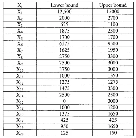
Lower and upper bounds of all the materials and products flowrate:

13

Table 3: Lower bound and upper bound of all material and products flow rate

x, Lower bound Upper bound

X! 12,500 15000

x2 ^{2000 2700}

x3 625 1100

X4 ^{1875 2300}

x5 ^{1700 1700}

x6 6175 9500

x7 1625 1950

x8 ^{2750 3300}

x9 ^{2500 3000}

Xio 3750 3000

Xi, 1000 1350

X12 1275 1275

Xi3 1475 3300

X14 2500 2500

X15 0 3000

X16 ^{1000 1200}

X17 ¹³⁷⁵ 1650

X18 425 425

X19 950 1650

X20 ^{125 150}

2 MONTE CARLO SIMULATION APPROACH BASED ON SAMPLE AVERAGE APPROXIMATION (SAA)

In this work, we adopt the Monte Carlo simulation approach for scenario generation based on the Sample Average Approximation (SAA) method (Shapiro, 2000;

Shapiro and Homem-de-Mello , 1998; You and Grossmann, 2008) proposed by Santoso et al. (2005). The procedure involved is as follows:

Stepl:

A relatively small number of scenarios (for example, 50 scenarios) with their associated probabilities are randomly and independently generated for the uncertain parameters of prices, demands, and yields. (This data is otherwise obtained from plant historical data.) The resulting stochastic model (a linear program) with the objective function given in (4) or (5) is solved to determine the optimal stochastic profit with its corresponding material flowrates.

14

max profit= E[z] =£ Z P*cvxi ~S P* ZZfe+SZw,M

iel seS seS te/ kzK /e/ meM

*[*,] ^[5]

E[z] = E[z0]-E&] (29)

Step 2:

From the stochastic profit in step 1 and materials's flowrate in step 1, Monte Carlo sampling variance estimator is calculated:

5("} K 5-1

Wherez^^c^x--^

• Confidence interval H of 1-a is given as:

zanS(n)

r -i , 2a/25(n)

I(*H-*.)J

_s=l

(30)

LJ Vs L J Vs

⁽³¹⁾

The minimum number of scenarios N that is theoretically required to obtain an optimal solution is determined using the relation below:

N =

Where:

H

~l2

(32)

Za/2 = 1-96 at confidence interval (1-a) = 95% (Assuming za/z is

standard normal deviate such that \-zal2 satisfies for a standard normal distributed variable z~N(0, 1), Pr(z^a/2) = 1-072

Numerical experiments indicate that well controlled choice of the sample sizes can significantly reduce the computational time and improve the accuracy of obtained

solutions.

15

Step 3:

Risk measure using the metrics of MAD and CVaR is incorporated in a new stochastic model with the scenarios given by the minimum number of scenarios N, in which the N number of scenarios are generated as a new set of independent random samples of the uncertain parameters.

A new stochastic model is formulated based on minimum number of scenarios N

with the incorporation of the risk measure of MAD and CVaR, respectively,

3. GENERAL FORMULATION OF STOCHASTIC REFINERY PLANNING WITH RISK EXPRESSED IN TERMS OF MAD

Konno and Koshizuka (2005), Konno and Yamazaki (1991), LI risk of mean- absolute deviation as a measure of deviation from the expected profit. Thus, the objective function of the model is reformulated as follow:

MAD(x) =£

n n

2>./*y

^{- E}

TRJXJ

>i . -'"' J

(33)

In our case, the rate of return R in (33) is replaced by unit price or unit cost of materials (crude oil and refinery products) and x refers to the production flow rate of materials in a refinery. Therefore, the formulation of the MAD term becomes:

MAD(z0) =£[|z0>,-£[z0][

= E

stS

YuPsZ0,t

StS

ZQ,s ~ / ,ftZ0..<

seS S€S

MAD(z0) =5>-

ssS (£/ fe/ SES

(34)

16

The expectation operator or mean of a discrete probability of deterministic profit is given by:

£[zo] =ZI A"V^ (35)

is/ seS

Where z0 =£c(i,*ff, (36)

isIP

Khor et al. 2007, MAD^ =£ P, x ^-£/>a

⁽³⁷⁾

se5 seS

where ^ = Z S ^A,* +S 2 fc^,*,* V5 e ^

iel keK iel meM

demand uncertainty penalty yield uncertainty penalty

4. GENERAL FORMULATION OF STOCHASTIC REFINERY PLANNING WITH RISK EXPRESSED IN TERMS OF CVAR

Rockafellar and Uryasev (2002) define Conditional Value-at-risk for continuous

distribution function:

Fa{x,VaR) =VaR+-l—\YL {f^9y^)-VaR) (38)

With discrete probability distribution in y, CVaR is written as:

Fa(x,VaR) =VaR +-^-Y,IJP^f^yi^-VaR)

I-a ,-e/ ssS-

<39)

Applying the concept of CVaR into the recourse terms:

max2 =£[z0]-eiCVaRZo-£,[^]-e3CVaR5

a) CVaRz : Risk measure for uncertainty in price of crude oil and refinery

products

CVaR(zJ =VaR, +-!_££A (C/A -VaR,) (40)

b) CVaR4: Risk measure for uncertainty in market demand and production

yield.

17

CVaR4-VaR2 +

l+«,?/' Z Z dukzi,s,k +Z Z ft>^-,5,m ~VaR2

i s / keK is/ msAf

(41) Put eq. (40) and (41) into (5), we achieve the stochastic model in which risk elements are expressed in term of CVaR.

CHAPTER 4

NUMERICAL RESULTS AND DISCUSSIONS

1. NUMERICAL RESULT

1.1 Determining minimum number of scenarios by Monte Carlo simulation approach based on the sample average approximation (SAA) technique to generate the scenarios

We illustrate the risk modeling approach proposed in this paper on the numerical example taken from Khor et al. (2008) and provide major details on the implementation using GAMS/CONOPT3.

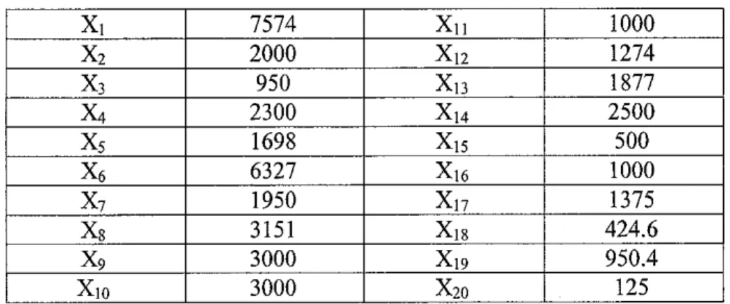
Table 4: Flowrates of crude oil and saleable products

Xi 7574 Xn 1000

x2 2000 X]2 1274

x3 ⁹⁵⁰ X13 1877

X4 2300 X14 2500

x5 1698 Xis ⁵⁰⁰

x6 ⁶³²⁷ Xi6 ¹⁰⁰⁰

x7 ¹⁹⁵⁰ Xn 1375

x8 ³¹⁵¹ Xi8 424.6

x9 ³⁰⁰⁰ X19 950.4

Xio 3000 X20 ¹²⁵

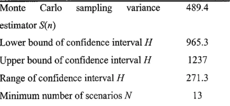
Table 5: Summary of computational results

Monte Carlo sampling variance 489.4 estimator S(n)

Lower bound of confidence interval H 965.3

Upper bound of confidence interval H 1237 Range of confidence interval H 271.3

Minimum number of scenarios N 13

19

1.2 Solving stochastic programming model to maximize profit with MAD as

risk measurement

z, = -8.02x, + 18.63x2 +8x3 + 12.46x4 +14.56x5 +6.05x6 -1.49x14 z2 =-7.97x, + 18.39x2 + 8.06x3 + 12.46x4 +14.4x5 +5.96x6 -1.5x14

(42) 2B = -8.01x, + 18.65x2 +8.O6X3 +12.59x4 + 14.48x5 + 6.01x6 -1.49x14

with probability: pi = 0.0038, p2 = 0.0986, ..., pi3 = 0.000752

The expectation of deterministic profit:

^[20] =(0.0038)(-8.02x] +18.63*, +8x3 +12.46x4 +14.56x5 +6.05xfl -1.49x]4) +(0.0986)(-7.97x, +18.39x, +8.06x3 +12.46x, +14.4xs +5.96x6 -1.5x14)

+

+(0.000752)(-8.01x1 +18.65x: +8.06x3 +12.59x4 +14.48x5 +6.01x6 -1.49xI4)

(43)

MAD(z0) =(0.0038)

•(0.0986)

(-8.02x, +18.63x, +8x3 +12.46x4 +14.56x; +6.05xfi -1.49xM)

(0.0038)(-8.02x, +18.63x, +8x3 +12.46x4 +14.56x5 +6.05x6 -1.49jcm)

+(0.0986) (-7.97*, +18.39x, +8.06x3 +12.46x4 +14.4x; +5.96x6 -1.5x]4)

_+.... +(0.000752) (-8.0U, +18.65x2 +8.06x3 +I2.59x4 +14.48x5 +6.01x6 - 1.49x14) (-7.97x, +18.39x3 +8.06x3 +12.46x4 +14.4x5 +5.96x6 -1.5x]4)

(0.0038)(-8.02x] +18.63x, +8x3 +12.46x4 +14.56x5 +6.05x6 -1.49x|4) +(0.0986)(-7.97X, +18.39x3 +8.06x3 +12.46x4 +14.4x5 +5.96x6 -1.5x14)

+.... +(0.000752)(-8.01xl +18.65x^ +8.06x3 +12.59x4 +14.48x5 +6.01x6 -1.49x|4)_

(-8.0b;, +18.65x2 +8.06x3 +12.59x4 +14.48x5 +6.01x6 -l-49x14)

(0.000752) (0.0038)(-8.02x, +18.63x2 +8x3 +12.46x4 +14.56x5 +6.05x6 -1.49x]4) +(0.0986)(-7.97x, +18.39x2 +8.06x3 +12.46x4 +14.4x5 +5.96x6 -1.5x14)

A-8.01x, +18.65x2 +8.06x3 +12.59x4 +14.48x5 +6.01x, A

-....+(0.000752)

-1.49x,

(44)

20

The expectation of the objective function value is given by the original objective fimction itself: The corresponding expression for expected profit is formulated for the 13 scenarios that have been randomly generated. Finally, computational results obtained from using GAMS/CONOPT3 gives a maximum profit of $681.95/day.

1.3 Solving stochastic programming to maximize profit with CVaR as risk

measurement

The following is the procedure for developing a loss distribution in order to determine the value for the parameter VaR.

• Determining VaRi from loss distribution of deterministic profit

The value-at-risk for uncertainty in prices of products and raw materials is named VaRi

• For each scenario, computing the deterministic profit by :

ielP

• The probability of each scenario is randomly generated using the Monte Carlo simulation method based on pseudorandom number generation.

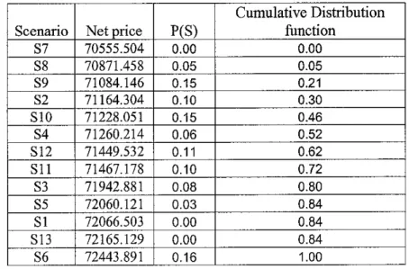
• The computed values zs are sorted in ascending order

Table 6: Deterministic profit and cumulative distribution function

Scenario Net price P(S)

Cumulative Distribution function

S7 70555.504 0.00 0.00

S8 70871.458 0.05 0.05

S9 71084.146 0.15 0.21

S2 71164.304 _0.10 0.30

S10 71228.051 0.15 0.46

S4 71260.214 0.06 0.52

S12 71449.532 0.11 0.62

Sll 71467.178 0.10 0.72

S3 71942.881 0.08 0.80

S5 72060.121 0.03 0.84

SI 72066.503 0.00 0.84

S13 72165.129 0.00 0.84

S6 72443.891 0.16 1.00

21

The plot of cumulative distribution function against the sorted deterministic profit values is developed to obtain a representation of the loss distribution. At confidence interval of (1-0!) = 0.95, we can read off the value of VaR} from the loss distribution plot, as depicted in Figures 3, which represents the penalty for uncertainty in prices and in both demands and yields, respectively

22

s.2

c

I 0.55

S 1

0.950.9

0.850.8

0.750.7-

0.65-

0.6

0.50.45-

0.4-

0.35-

0.3-

0.25-

0.20.15

0.1-

0.05-

070000 LossDistributionforUncertaintyinPrices

70500710007150072000

rtcjllfdD:Deterministicprofitduetouncertaintyinprices _^_

7250073000

From Figure 3, at (1-a) = 0.95, VaRi = 7.235E+4

• Determining VaR2 from loss distribution by demand and yield penalty.

Similar to the procedure for determining VaR], the following is the procedure for developing a loss distribution in order to determine the value for the parameter VaR2:

• For each scenario, penalty of market demand for products and production yield is calculated:

^ =E Z di,kZi,s,k +Z S aUmyi,s,m V5 £S

iel keK iel meM

• The computed values of ^s are sorted in ascending order. The cumulative distribution function for each scenario is developed:

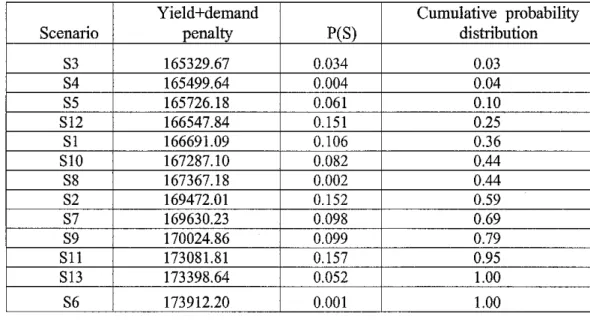
Table 7: Penalty of yield and demand and cumulative distribution function

Scenario

Yield+demand

penalty P(S)

Cumulative probability

distribution

S3 165329.67 0.034 0.03

S4 165499.64 0.004 0.04

S5 165726.18 0.061 0.10

S12 166547.84 0.151 0.25

SI 166691.09 0.106 0.36

S10 167287.10 0.082 0.44

S8 167367.18 0.002 0.44

S2 169472.01 0.152 0.59

S7 169630.23 0.098 0.69

S9 170024.86 0.099 0.79

Sll 173081.81 0.157 0.95

S13 173398.64 0.052 1.00

S6 173912.20 0.001 1.00

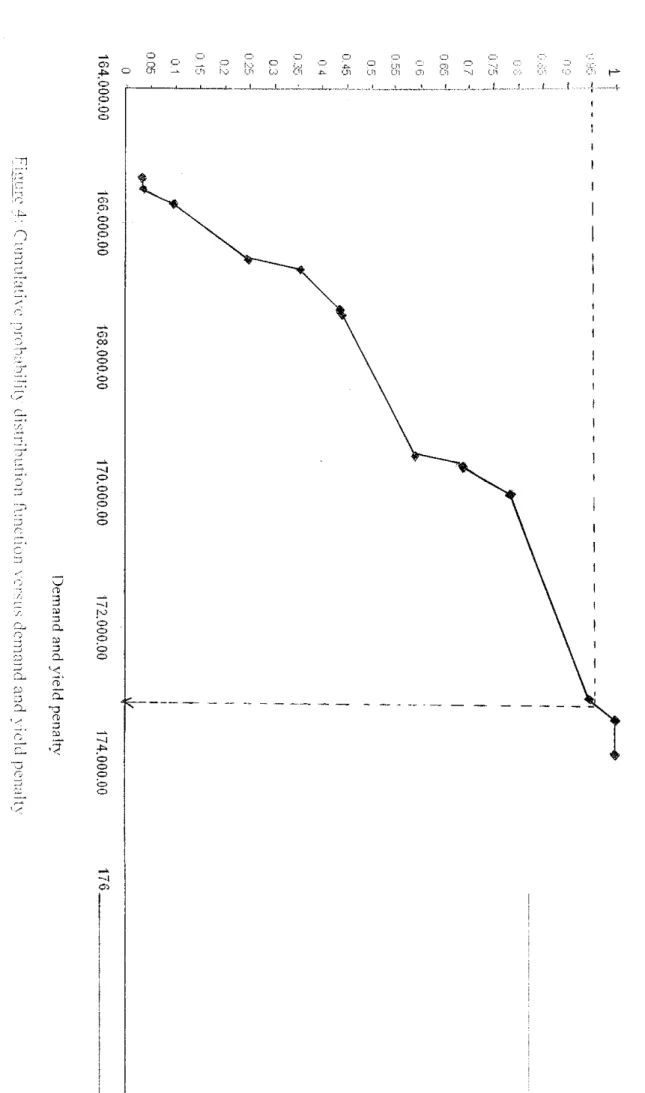
The cumulative distribution function is plotted against the sorted computed values to obtain a representation of the loss distribution.

At confidence interval of (1-a) = 0.95, we can read off the value of VaR2 from the loss distribution plot, as depicted in Figures 4, which represents the penalty for uncertainty in prices and in both demands and yields, respectively.

24

Cumulativeprobjhi

-•i-UnbuiKin!ii!ie!!'."':

164.000.00166.000.00168.000.00170.000.0072.000.00174.000.00

Demandandyieldpenalty

Figure4:CtmiulaMvcproK'HHHdistributionfunclionvo^usdemandand\idt.1penahv 176.

From Figure 4, at (1-ot) - 0.95, Var2 = 1.731E+5

From VaRi and vaR2 values, apply model in eq. (5) in Gams, (Profit)r

$20,820.665/day

Summary of the numerical result

Table 8: (Values of) Parameters

Goal programming weight for risk measure on price uncertainty

0.0001

Goal programming weight for risk measure on demand and yield uncertainty

0.01

Confidence level p ^0.95

Table 9: Computational results

Optimal solution for model with MAD $681.95/day

VaRi 7.235E+4

VaR2 1.731E+5

Optimal solution for model with CVaR $20 800.66/day Expected profit E[zq] for model with CVaR $23343.776/day

Table 10: Computational statistics of GAMS implementation for determining optimal solutions of MAD- and CVaR-based mean-risk stochastic program

Solver

Number of continuous variables

Number of constraints

CPU time/resource usage

Number of iterations

26

GAMS/CONOPT3 281

145

(trivial)

20 (using MAD) 101 (using CVaR)

Table 11: Model statistics Number of continuous variables 281

Number of constraints 145

Table 12: Model performance

Solver

CPU time/resource usage

Number of iterations

2. DISCUSSION

GAMS/CONOPT3

(trivial)

20 (using MAD) 101 (using CVaR)

Table 13: Comparison between MAD and CVaR

Factor MAD CVaR

1. Considers confidence level

(95%, 99%, etc..)

No Yes

2. Differentiates distribution of

objective function (whether discrete or continuous)

No Yes

3. Computational property Hon-.:

HnzaAs

Linear. Applicable to large portfolios

& large number of scenarios with little computational resources

From Table 13, we see that CVaR is more advantageous than MAD because the

former takes into account the confidence level and the class of distribution of the

objective function (whether it is a discrete or continuous distribution). Moreover, the actual form of MAD is nonlinear (although it can be linearized, for example, as

proposed by Papahristodoulou and Dotzauer (2004)) while CVaR is a linear

27

function. Furthermore, in the case of a large number of scenarios, but with the availability of limited computational resource, CVaR is more useful than MAD.

28

CHAPTER 5

CONCLUSIONS AND RECOMMENDATIONS

1. CONCLUSIONS

Stochastic programming is one of the ultimate operation research models for optimization that involves uncertainties. The input values such as materials flowrate, shortfall and surplus of demand and yield penalty are determined maximize the profit.

Monte Carlo simulation approach based on Sample Average Approximation (SAA) is a powerful method to estimate the minimum number of scenarios required to compute the optimal solution, because it can capture all the possible scenarios and is thus representative of all scenarios. This procedure saves time and is convenient particularly if a large number of scenarios have been sampled. In this work, for the risk metric of MAD, we have verified that the same optimal solution as for the mean-risk stochastic model with 13 scenarios is obtained if larger numbers of scenarios are considered, for instance, for 100 and 300 scenarios. A similar experiment on CVaR is currently ongoing.

This work attempts to consider the use of the risk metrics of MAD and CVaR for the explicit handling of economic and operational risk management in refineryplanning problems under uncertainty in prices, demands, and yields.

The risk is expressed in form of Mean Absolute Deviation - a measure of operational risk provides the computational non-linear property. However, the non linear property can be linearised.

Conditional Value-at Risk used in conjunction with Value- at Risk is convenient for large portfolios and a large number of scenarios with relatively small computation

29

resources. Moreover, CVaR is a convex function. In petroleum refinery planning,

the recourse term is written in form of CVaR.

Conditional Value-at Risk is more advantageous than Mean Absolute Deviation because Conditional Value-at Risk consider the confidence interval, the distribution of objective function (discrete or continuous)

2. RECOMMENDATIONS

The recommendations for future studies on the work presented here include the following:

• To develop a systematic approach for considering the weight factors B\ and 82 in the stochastic programming framework.

• To develop an approach for obtaining the Pareto-optimal curve for a mean- risk stochastic program with MAD and CVaR as risk measures.

30

REFERENCES

1. R. B. Webby, P. T. Adamson, J. Boland, P. G. Howlett, A. V. Metcalfe, and J. Piantadosi, 2007, The Mekong—applications of value at risk (VaR) and conditional value at risk (CVaR) simulation to the benefits, costs, and consequences of water resources development in a large river basin, Ecological Modeling, 201, 89-96.

2. R. T. Rockafellar and S. Uryasev, 2000, Optimization of conditional value- at-risk, Journal of Risk, 2, 3, 21-41.

3. R. T. Rockafellar and S. Uryasev, 2002, Conditional Value-at-Risk for general loss distributions, Journal of Banking and Finance, 26, 7: 1443-

1471.

4. C. S. Khor, A. Elkamel, K. Ponnambalam, and P. L. Douglas, 2008, Two- Stage Stochastic Programming with Fixed Recourse via Scenario Planning with Financial and Operational Risk Management for Petroleum Refinery Planning under Uncertainty, Chemical Engineering and Processing, 47, 9-

10,1744-1764.

5. Konno, H. and H. Yamazaki, Mean Absolute Deviation Portfolio Optimization Model and Its Application to Tokyo Stock Market.

Management Science. 37, 519-531, 1991

6. H.M Markowitz, Portfolio selection, J. Finance 7(1) (1952)77-91

7. Rockafellar R.T. and S. Uryasev , Conditional Value-at- Risk for General Loss Distributions. Research Report 2001-5. ISE Dept, University of Florida, April 2001

8. You, F., J. M. Wassick, and I. E. Grossmann. Risk management for a global supply chain planning under uncertainty: models and algorithms [textfile].

Retrieved September 26, 2008 from the World Wide Web:

http://egon.cheme.cmu.edu/Papers/RiskMgmtDow.pdf

9. Fengqi You and John M. Wassick, Ignacio E. Grossmann , Risk Management for a Global Supply Chain Planning under Uncertainty: Model and Algorithms, 2008

31

10. Norbert J. Jobst and Stavros A. Zenios, The Tail That Wags the Dog:

Integrating Credit Risk in Asset Portfolios

11. Shapiro, A. and T. A. Homem-de-Mello. A simulation-based approach to two-stage stochastic programming with recourse. Mathematical Programming %1 (1998): 301-325.

12. Shapiro, A., 2000, Stochastic Programming by Monte Carlo Simulation Methods, Stochastic Programming E-Prints Series, Retrieved February 10, 2007 from the World Wide Web: http://www.isye.gatech.edu/%7Eashapiro/

publications/SBOsurvey.pdf

13. Al-Sharrah. Ghanima. Planning the petrochemical industry in Kuwait using economic and safety objectives. PhD Thesis. Loughborough University,

2006.

32

APPENDIX

1. PROGRAM CODE

*STITTLE: FINDING THE NUMBER OF SCENARIO

SETS 1 material /1*20/

M YEILD SHOREALL OR SURPLUS /Ml , M2/

K DEMAND SHORT FALL OR SURPLUS /Kl, K2/

Sonecho >taskin.txt

dset=S mg=Sheet4!A16:A28 rdim=l dset=IDmg=Sheet4!B15:F15 cdim=l dset=IYrng=Sheet4!H15:L15 cdim-1 dset=IPrng=Sheet4!N15:T15 cdim^l pai=D rng=Sheet4!A15:F28 cdim=l rdim=l par=Yieldmg=Sheet4!G15:L28 cdim=l rdim=l par=Price rag=Sheet4!M15:T28 cdim=l rdim=l par=Prng=Sheet4!U15:V28 rdim=l

Soffecho

Scall gdxxnv.exe CVaR.xls @taskin.txt

Sgdxin CVaR.gdx

Sets S(*) scenario ID(I) demand IY(I) yeild IP(I) price;

Sload S ID IY IP display S, ID, IY, IP;

Parameters D(S,ID) demand Yield(S,IY) yield Price(S,IP) price P(S) probability Sload D Yield Price P display D, Yield, Price , P;

Sgdxin

Table Penalty_Demand<ID,K) TABLE OF PENALTY DEMAND

Kl K2

2 25 20

33

3 17 13

4 5 4

5 6 5

6 10 8;

Table Penalty_Yield(IY,M) TABLE OF PENALTY YIELD

Ml M2

7 5 3

4 5 4

8 5 3

9 5 3

10 5 3;

Variables

OBJ Maximize Profit for Z {objective function value) Varl

Var2 X(I);

Positive Variables

Y(IY,S,M) SHORT FALL OR SURPLUS FOR YEILD Z(ID,S,K) SHORT FALL OR SURPLUS FOR DEMAND

Equations

OBJFNC Objective function DEMAND(ID,S) Demand, YIELD_CON(IY,S) Yield, Feedi,

Feed 14, PDUJ4J6, PDUJ4J7, PDU_14_20, FB_2_11, FB_2J6, FB_5J2, FB_5_18, UB_8, UBJ4, UB_17, UB_18, UB 6

OBJFNC. OBJ =e= SUM«S,IP),P(S)*PRICE(S,IP)*X(IP)) -0.0001 *(72400+ (l/(i- 0.95))*SUM((S,IP),P(S)*(PRICE(S,IP)*X(IP)-72400)))-

SUM(S,P(S)*(SUM((ID,K),Penalty_Demand(ID,K)*Z(ID,S,K))+SUM((IY,M),Penalty_Yield(IY,M)*Y(IY,S,M)))).

0.01*( 173200

+ (1/(1 0.95))*SUM(S,P(S)*(SUM((ID,K), Penalty_Demand(ID,K)*Z(ID,S,K)) +SUM((IY,M),PenaIty_Yield(IY,M)*Y(IY,S,M))-173200)));

34

♦•LIMITATIONSOF PLANT CAPACITY FeedL. X(T)=L= 15000;

Feedl4.. X('14')=L=2500;

*Reformulated stochastic constraints to account for uncertain yield coefficient

YIELD_CON(IY,S).. -YIELD(S,IY)*X('r} + X(IY) + Y(IY,S;Mr) - Y(IY,S,'M2') =E= 0;

**CONSTRAINTS ON PRODUCTION DEMANDS

DEMAND(ID,S).. X(ID) + Z(ID,S,'K r)-Z(ID,S,'K2') =E= D(S,ID);

PDU_14_16.. -0.40*X('14,) + X(,16')=E=0;

PDUJ4J7.. -0.55*X('14') + X('17')=E=0;

PDU_14_20.. -0.05*X('34') + X('20') =E- 0;

FB_2_11.. 0.5*X('2') -X('ll') =E= 0;

FB_2_16.. 0.5*X('2') - X('16') =E= 0;

FB__5_12.. 0.75*X('5') - X('12') =E= 0;

FB_5_18.. 0.25*X('5')-X('18')=E=0;

UB_8- -X('7') + X('3') + X('l 3') =E= 0;

UBJ4.. -X('8') + X('12') + X('I3') =E= 0;

UBJ7.. -X('9') + X('14') + X('I5') =E= 0;

UB_18.. -X('17') + X('18') +X('19') =E= 0;

UB_6.. -X('IO') - X('13') -XC15') - X('19') + X('6') =E= 0;

*DECISION VARIABLE BOUNDS

Y.UP(IY,S,M)=1500;

* Initial values X.L{T)= 12500;

X.L{'2') = 2000;

X.L{'3') = 625;

X.L('4')=1875;

X.L('5')=1700;

X.L('6') = 6175;

X.L('7')=1625;

X.LC81) = 2750;

X.L('9') = 2500;

X.L('10,)-3750 X.L('ir) = 1000 X.L('12')=1275 X.L('13')=1475 X.L('14') = 2500 X.L('15') = 0;

X.L('16')=1000;

X.L('17') = 1375;

X.L('I8') = 425;

X.L('19') = 950;

X.L('20')=125;

Upper bounds of variables

35

X.UP('1') = X.UP(T) = X.UP('3') - X.UP('4') = X.UP('5') = X.UP('6') = X.UP('7') = X.UP('8') = X.UP('9') = X.UPCIO1) x.up('ir) X.UP('12') X.UP('I3') X.UP('14') X.UP('15') X.UP('lff) X.UPC1T) x.upcis') x.upc^*) X.UP{'20')

15000 2700 1100 2300 1700 9500 1950 3300 3000

= 3000

= 1350

= 1275

= 3300

= 2500

= 3000

= 1200

= 1650

= 425;

= 1650;

= 150;

MODEL CVaR /al!/;

SOLVECVaR USINGLP MAXIMIZING OBJ;

DISPLAY OBJ.L, X.L, Y.L, Z.L ; EXECUTE_UNLOAD 'CVaR.GDX'.OBJ;

EXECUTE 'GDXXRW.EXE CVaR.GDX VAR=OBJ RNG=SHEET4!A68':

2. EXPECTED PROFIT

S O L V E

HODEL FindEprofit

TYPE LP SOLVER CPLEX

S U H H A R Y

OBJECTIVE E_profit

DIRECTION MAXIMIZE FROM LINE 118

**** SOLVER STATUS

**** MODEL STATUS

**** OBJECTIVE VALUE

1 NORMAL COMPLETION 1 OPTIMAL

1100.9109

36

3. VARIANCE ESTIMATOR

S O L V E

MODEL FindSn_Sn

TYPE DNLP SOLVER CONOPT

S U M M A R Y

OBJECTIVE Sn DIRECTION MINIMIZE FROM LINE 143

'*** SOLVER STATUS

'*** MODEL STATUS '*** OBJECTIVE VALUE

1 NORMAL COMPLETION

2 LOCALLY OPTIMAL 503.0991

4. MAXIMUM PROFIT WITH MAD AS RISK MEASUREMENT

**** REPORT SUMMARY : 0 NONOPT 0 INFEASIBLE 0 UNBOUNDED

0 ERRORS

•GAMS Rev 146 XS6/MS Windows 02/19/05 10:07:35 Page G e n e r a l A l g e b r a i c M o d e l i n g S y s t e m

E x e c u t i o n

2 00 VARIABLE OBJ.L SSI.954 Maximize Profit for Z

(objective function v alue)

5. MAXIMUM PROFIT WITH CVAR AS RISK MEASUREMENT

**** REPORT SUHHARY : 0 NONOPT 0 INFEASIBLE 0 UNBOUNDED

JGAHS Rev 146 XS6/HS Windows 03/23/05 15:35:02 Page G e n e r a l A l g e b r a i c M o d e l i n g S y s t e m

E x e c u t i o n

213 VARIABLE OBJ.L

37

20320.665 Haximise P r o f i t for Z (objective function v alue)

6. MATERIALS' FLOWRATE

204 VARIABLE X.L

I 7574.363, 2 2000.000, 3 950.000, 4 2300.000, 5 1689.393 6 633 6.419, 7 1950.000, 8 3150.813, 9 3000.000, 10 3000.000 II 1000.000, 12 1267.045, 13 1883.768, 14 2500.000, 15 500.000 16 1000.000, 17 1375.000, 18 422.348, 19 952.652, 20 125.000

38