new families of universal portfolios and their

NEW FAMILIES OF UNIVERSAL PORTFOLIOS AND THEIR PERFORMANCES

By

KUANG KEE SENG

A thesis submitted to the

Department of Mathematical and Actuarial Sciences, Lee Kong Chian Faculty of Engineering and Science,

Universiti Tunku Abdul Rahman,

in partial fulfillment of the requirements for the degree of Doctor of Philosophy (Science)

August 2022

ABSTRACT

NEW FAMILIES OF UNIVERSAL PORTFOLIOS AND THEIR PERFORMANCES

KUANG KEE SENG

In the world of investment, various types of investment product are available for the investor to seek for long term investment return. These products include invest in real-estate, invest in foods and beverages, invest in bonds, invest in commodities and many more. Choosing the ’right’ asset to invest is difficult.

Losses can occur if the chosen asset behaves in an unfavourable way. In the modern era, investors use portfolio in their investment strategy. A portfolio is a combination or collection of a series of financial instruments like commodities, bonds, stocks, cashes and etc. It is a method that commonly spotted in the market which it can reduce the risk significantly by not allocating all the capital into one basket. Portfolio helps to diversify the investor capital and allocate those wealth onto various options to prevent occurrence of huge loss due to unpleasant event. As an individual investor, we need to determine the optimum allocation for each of the components in the portfolio. A well-diversified portfolio is crucial for any investor to yield a higher return.

Universal portfolio is a strategy of trading on stocks that does not assume any probability model for the stock prices. Universal portfolio is an investment technique where it helps us to generate portfolio vector to produce high wealth return in a long run.

In this research, new possible ways to generate new universal portfolios are studied. Objective functions with different divergence have been tested to obtain the new universal portfolios. The purpose is to obtain the next-day stocks’ allocation of the portfolio which could maximize the wealth return.

Next, the performance of the newly derived universal portfolios is studied by running these universal portfolios on some selected stocks from the Kuala Lumpur Stock Exchange (KLSE). These results will be compared with others and the performances are studied intensively.

Beside comparing the performances, a new family of universal portfolios is developed. Most of the newly derived universal portfolios are linked to the universal portfolio generated by f-divergence and universal portfolio generated by Bregman divergence. These two universal portfolios are the general form of Helmbold universal portfolio.

For numerical experiment of the performance of universal portfolio, it is shown that the newly derived universal portfolios can perform as good as Helmbold universal portfolio. The results of these universal portfolios show that it is possible to increase the wealth of the investor by using these portfolios in investment.

ACKNOWLEDGEMENTS

I would like to acknowledge and give my appreciation to my main supervisor, Dr. Koh Siew Khew and co-supervisor, Dr. Goh Yann Ling who made this work possible. Their advice and guidance carried me through all the stages of writing my projects.

I would also like to thank the committee members from the faculty for letting my proposal defense to be an enjoyable moment, and provided me with brilliant comments and suggestions.

I would also like to give special thanks to my wife, Ms. Wan Mei Er and my family as a whole for their continuous support and understanding when undertaking my research and writing my project. I would also like to specially thank to my late-father, who always encouraged and guided me to be a better man.

I would also like to give my utmost appreciation to Dr. Tan Choon Peng for his guidance. He taught me patiently throughout my research to allow me to gain more understandings on this topic.

Lastly, I would like to thank my friends, especially Mr. Chew Chun Yong, Dr. Lee Min Cherng and Mr. Gabriel for providing me valuable information and knowledge.

APPROVAL SHEET

This thesis entitled “NEW FAMILIES OF UNIVERSAL PORTFOLIOS AND THEIR PERFORMANCES” was prepared by KUANG KEE SENG and submitted as partial fulfilment of the requirements for the degree of Doctor of Philosophy (Science) at Universiti Tunku Abdul Rahman.

Approved by:

(Dr KOH SIEW KHEW) Date: ...

Assistant Professor

Department of Mathematical and Actuarial Sciences Lee Kong Chian Faculty of Engineering and Science Universiti Tunku Abdul Rahman

(Dr GOH YANN LING) Date: ...

Assistant Professor

Department of Mathematical and Actuarial Sciences Lee Kong Chian Faculty of Engineering and Science Universiti Tunku Abdul Rahman

10/08/2022 10/08/2022

LEE KONG CHIAN FACULTY OF ENGINEERING AND SCIENCE UNIVERSITI TUNKU ABDUL RAHMAN

Date: 10 AUGUST 2022

SUBMISSION OF THESIS

It is hereby certified that KUANG KEE SENG (ID No: 14UED07966) has completed this thesis entitled “NEW FAMILIES OF UNIVERSAL PORTFOLIOS AND THEIR PERFORMANCES” under the supervision of Dr KOH SIEW KHEW (Supervisor) from the Department of Mathematical and Actuarial Sciences, Lee Kong Chian Faculty of Engineering and Science, and Dr GOH YANN LING (Co-Supervisor) from the Department of Mathematical and Actuarial Sciences, Lee Kong Chian Faculty of Engineering and Science.

I understand that the University will upload a softcopy of my thesis in PDF format into UTAR Institutional Repository, which may be accessible to UTAR community and public.

Yours truly,

(KUANG KEE SENG)

Type text here

DECLARATION

I, KUANG KEE SENG hereby declare that the thesis is based on my original work except for quotations and citation which have been duly acknowledged. I also declare that it has not been previously or concurrently submitted for any other degree at UTAR or other institutions.

(KUANG KEE SENG)

Date: ^10/8/2022

TABLE OF CONTENTS

Page

ABSTRACT ii

ACKNOWLEDGEMENTS iv

APPROVAL SHEET v

SUBMISSION SHEET vi

DECLARATION vii

LIST OF TABLES xvii

LIST OF ABBREVIATIONS xviii

CHAPTER

1 INTRODUCTION 1

1.1 Objective 2

1.2 Literature Review 2

1.3 Thesis Overview 5

1.4 Definitions 7

1.4.1 Some Preliminaries 7

1.4.2 Objective Function 8

2 DATA COLLECTION 10

2.1 Bursa Malaysia 10

2.2 Stocks Selection 11

2.3 Stock Data Sets 12

3 UNIVERSAL PORTFOLIO GENERATED BY

ZERO-GRADIENT SET OF LOGARITHM OBJECTIVE

FUNCTION 14

3.1 Reciprocal-Price-Relative (RPR) Universal Portfolio 14

3.1.1 Type 1 RPR Universal Portfolio 15

3.1.2 Type 2 RPR Universal Portfolio 22

3.2 Universal Portfolio Generated by R´enyi and Generalized

Kullback-Leibler Divergence 28

3.2.1 Universal Portfolio Generated by R´enyi Divergence 29 3.2.2 Universal Portfolio Generated by Generalized Kullback-

Leibler Divergence 31

3.3 Reverse Helmbold Universal Portfolio 41

4 f-DIVERGENCE AND ITS REVERSE 48

4.1 f-Divergence 48

4.1.1 TypekUniversal Portfolio Generated by f-Divergence 48

4.2 Reverse f-divergence 58

5 STRONG FORM AND WEAK FORM OF f-DIVERGENCE 63

5.1 Bregman Divergence 63

5.1.1 Universal Portfolio Generated by Bregman Divergence 63 5.1.2 Universal Portfolio Generated by Reverse Bregman

Divergence 71

5.2 f-Disparity Difference 73

5.2.1 Universal Portfolio Generated by f-disparity difference 74 5.2.2 Universal Portfolio Generated by Rational Function 80

6 CONCLUSION 88

6.1 Summary 88

6.2 Future Works 90

LIST OF REFERENCES 94

LIST OF PUBLICATIONS 96

APPENDICES 97

LIST OF TABLES

Table Page

2.1 List of Malaysian companies in data sets D, E, F, G and H 12 2.2 List of Malaysian companies in data sets J, K, L, M and N 13 3.1 The wealth S₁₅₀₀ and the final portfolio b₁₅₀₁ achieved by the

Type 1 RPR universal portfolio for stock data set D after 1500 trading days, where the initial portfoliob1= (0.2,0.2,0.2,0.2,0.2) 19 3.2 The wealth S₁₅₀₀ and the final portfolio b₁₅₀₁ achieved by the

Type 1 RPR universal portfolio for stock data set E after 1500 trading days, where the initial portfoliob₁= (0.2,0.2,0.2,0.2,0.2) 19 3.3 The wealth S1500 and the final portfolio b1501 achieved by the

Type 1 RPR universal portfolio for stock data set F after 1500 trading days, where the initial portfoliob₁= (0.2,0.2,0.2,0.2,0.2) 20 3.4 The wealth S₁₅₀₀ and the final portfolio b₁₅₀₁ achieved by the

Type 1 RPR universal portfolio for stock data set G after 1500 trading days, where the initial portfoliob₁= (0.2,0.2,0.2,0.2,0.2) 20 3.5 The wealth S₁₅₀₀ and the final portfolio b₁₅₀₁ achieved by the

Type 1 RPR universal portfolio for stock data set H after 1500 trading days, where the initial portfoliob1= (0.2,0.2,0.2,0.2,0.2) 21 3.6 The wealth S₁₅₀₀ and the final portfolio b₁₅₀₁ achieved by the

pseudo relaxed Type 2 RPR universal portfolio for stock data set D after 1500 trading days, where the initial portfolio b1 =

(0.2,0.2,0.2,0.2,0.2) 25

3.7 The wealth S₁₅₀₀ and the final portfolio b₁₅₀₁ achieved by the pseudo relaxed Type 2 RPR universal portfolio for stock data set E after 1500 trading days, where the initial portfolio b1 =

(0.2,0.2,0.2,0.2,0.2) 26

3.8 The wealth S₁₅₀₀ and the final portfolio b₁₅₀₁ achieved by the pseudo relaxed Type 2 RPR universal portfolio for stock data set F after 1500 trading days, where the initial portfolio b1 =

(0.2,0.2,0.2,0.2,0.2) 26

3.9 The wealth S₁₅₀₀ and the final portfolio b₁₅₀₁ achieved by the pseudo relaxed Type 2 RPR universal portfolio for stock data set G after 1500 trading days, where the initial portfolio b1 =

(0.2,0.2,0.2,0.2,0.2) 27

3.10 The wealth S₁₅₀₀ and the final portfolio b₁₅₀₁ achieved by the pseudo relaxed Type 2 RPR universal portfolio for stock data set H after 1500 trading days, where the initial portfolio b1 =

(0.2,0.2,0.2,0.2,0.2) 27

3.11 The wealth S₁₅₀₀ and the final portfolio b₁₅₀₁ achieved by the pseudo relaxed R´enyi universal portfolio for stock data set D after 1500 trading days, where the initial portfolio b₁= (0.2,0.2,0.2,0.2,0.2),α=10 andβ =6. 36 3.12 The wealth S₁₅₀₀ and the final portfolio b₁₅₀₁ achieved by the

pseudo relaxed R´enyi universal portfolio for stock data set E after 1500 trading days, where the initial portfolio b₁= (0.2,0.2,0.2,0.2,0.2),α=10 andβ =6. 37 3.13 The wealth S₁₅₀₀ and the final portfolio b₁₅₀₁ achieved by the

pseudo relaxed R´enyi universal portfolio for stock data set F after 1500 trading days, where the initial portfolio b₁= (0.2,0.2,0.2,0.2,0.2),α=10 andβ =6. 37 3.14 The wealth S₁₅₀₀ and the final portfolio b₁₅₀₁ achieved by the

pseudo relaxed R´enyi universal portfolio for stock data set G after 1500 trading days, where the initial portfolio b₁= (0.2,0.2,0.2,0.2,0.2),α=10 andβ =6. 37

3.15 The wealth S₁₅₀₀ and the final portfolio b₁₅₀₁ achieved by the pseudo relaxed R´enyi universal portfolio for stock data set H after 1500 trading days, where the initial portfolio b₁= (0.2,0.2,0.2,0.2,0.2),α=10 andβ =6. 38 3.16 The wealth S₁₅₀₀ and the final portfolio b₁₅₀₁ achieved by the

pseudo relaxed Kullback-Leibler universal portfolio for stock data set D after 1500 trading days, where the initial portfolio b₁= (0.2,0.2,0.2,0.2,0.2),α=0.1 andβ =2. 39 3.17 The wealth S₁₅₀₀ and the final portfolio b₁₅₀₁ achieved by the

pseudo relaxed Kullback-Leibler universal portfolio for stock data set E after 1500 trading days, where the initial portfolio b₁= (0.2,0.2,0.2,0.2,0.2),α=0.1 andβ =2. 39 3.18 The wealth S₁₅₀₀ and the final portfolio b₁₅₀₁ achieved by the

pseudo relaxed Kullback-Leibler universal portfolio for stock data set F after 1500 trading days, where the initial portfolio b₁= (0.2,0.2,0.2,0.2,0.2),α=0.1 andβ =2. 40 3.19 The wealth S₁₅₀₀ and the final portfolio b₁₅₀₁ achieved by the

pseudo relaxed Kullback-Leibler universal portfolio for stock data set G after 1500 trading days, where the initial portfolio b₁= (0.2,0.2,0.2,0.2,0.2),α=0.1 andβ =2. 40 3.20 The wealth S₁₅₀₀ and the final portfolio b₁₅₀₁ achieved by the

pseudo relaxed Kullback-Leibler universal portfolio for stock data set H after 1500 trading days, where the initial portfolio b₁= (0.2,0.2,0.2,0.2,0.2),α=0.1 andβ =2. 41 3.21 The wealth S₁₅₀₀ and the final portfolio b₁₅₀₁ achieved by the

reverse Helmbold universal portfolio for stock data set D after 1500 trading days, where the initial portfolio

b₁= (0.2,0.2,0.2,0.2,0.2) 45

3.22 The wealth S₁₅₀₀ and the final portfolio b₁₅₀₁ achieved by the reverse Helmbold universal portfolio for stock data set E after 1500 trading days, where the initial portfolio

b₁= (0.2,0.2,0.2,0.2,0.2) 46

3.23 The wealth S₁₅₀₀ and the final portfolio b₁₅₀₁ achieved by the reverse Helmbold universal portfolio for stock data set F after 1500 trading days, where the initial portfolio

b₁= (0.2,0.2,0.2,0.2,0.2) 46

3.24 The wealth S₁₅₀₀ and the final portfolio b₁₅₀₁ achieved by the reverse Helmbold universal portfolio for stock data set G after 1500 trading days, where the initial portfolio

b₁= (0.2,0.2,0.2,0.2,0.2) 46

3.25 The wealth S₁₅₀₀ and the final portfolio b₁₅₀₁ achieved by the reverse Helmbold universal portfolio for stock data set H after 1500 trading days, where the initial portfolio

b₁= (0.2,0.2,0.2,0.2,0.2) 47

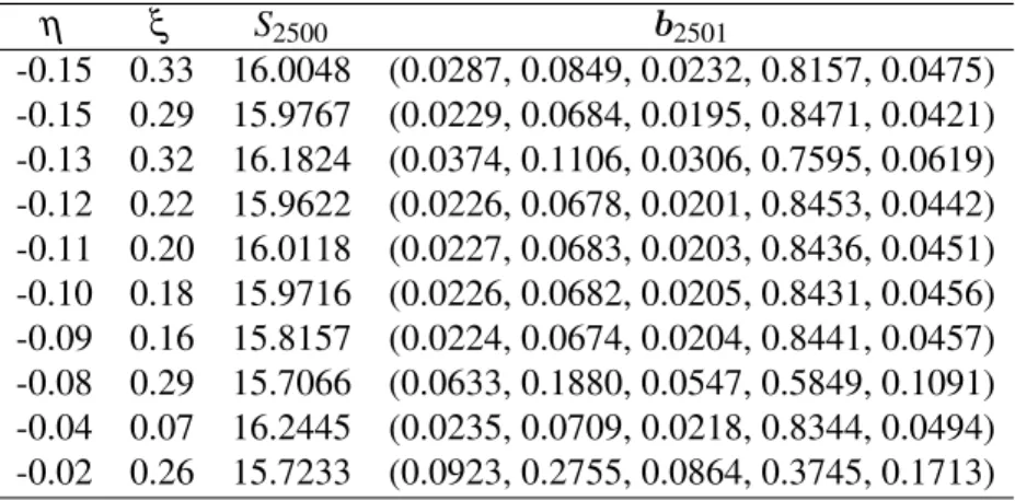
4.1 The wealthS₂₅₀₀achieved after 2500 trading days by running the Type 1 Helmbold portfolio over the data set J for selected value ofη together with final portfoliob2501 54 4.2 The wealthS₂₅₀₀achieved after 2500 trading days by running the

Type 1 Helmbold portfolio over the data set K for selected value ofη together with final portfoliob2501 54 4.3 The wealthS2500achieved after 2500 trading days by running the

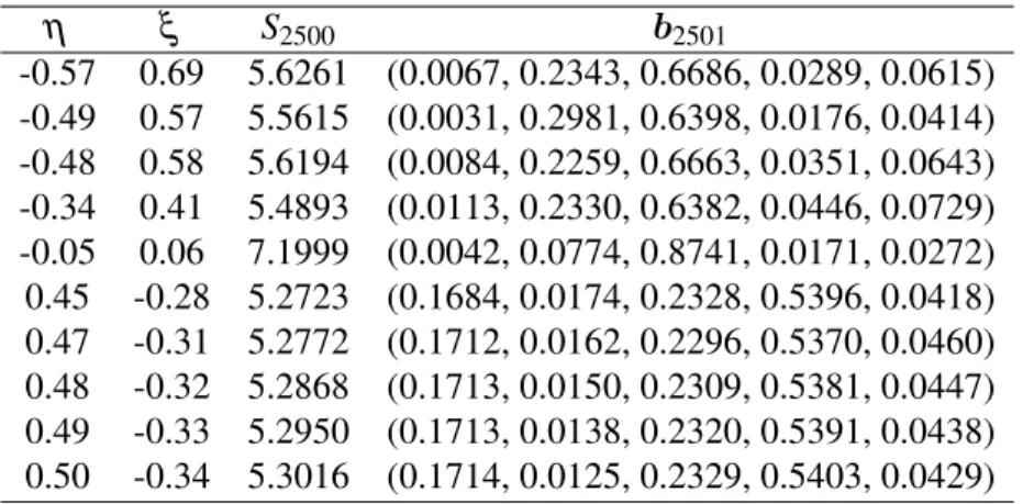
Type 1 Helmbold portfolio over the data set L for selected value ofη together with final portfoliob2501 54 4.4 The wealthS₂₅₀₀achieved after 2500 trading days by running the

Type 1 Helmbold portfolio over the data set M for selected value ofη together with final portfoliob2501 55

4.5 The wealthS₂₅₀₀achieved after 2500 trading days by running the Type 1 Helmbold portfolio over the data set N for selected value ofη together with final portfoliob2501 55 4.6 The wealthS₂₅₀₀achieved after 2500 trading days by running the

Type 2 Helmbold portfolio over the data set J for selected value ofη andη =0.8 together with final portfoliob2501 55 4.7 The wealthS2500achieved after 2500 trading days by running the

Type 2 Helmbold portfolio over the data set K for selected values ofη andγ =0.4 together with final portfoliob2501 56 4.8 The wealthS₂₅₀₀achieved after 2500 trading days by running the

Type 2 Helmbold portfolio over the data set L for selected values ofη andγ =0.1 together with final portfoliob2501 56 4.9 The wealth S₂₅₀₀ achieved after 2500 trading days by running

the Type 2 Helmbold portfolio over the data set M for selected values ofη andγ=0.3 together with final portfoliob2501 57 4.10 The wealthS₂₅₀₀achieved after 2500 trading days by running the

Type 2 Helmbold portfolio over the data set N for selected values ofη andγ =0.1 together with final portfoliob2501 57 5.1 The wealth S2500 and the final portfolio b2501 achieved by the

Universal Porfolio generated by Bregman Divergence for data set J ,where the initial portfoliob₁= (0.2,0.2,0.2,0.2,0.2)and

β =0.01. 68

5.2 The wealth S2500 and the final portfolio b₂₅₀₁ achieved by the Universal Porfolio generated by Bregman Divergence for data set K ,where the initial portfoliob₁= (0.2,0.2,0.2,0.2,0.2)and

β =0.001. 68

5.3 The wealth S₂₅₀₀ and the final portfolio b₂₅₀₁ achieved by the Universal Porfolio generated by Bregman Divergence for data set L ,where the initial portfoliob1= (0.2,0.2,0.2,0.2,0.2)and

β =0.01. 69

5.4 The wealth S₂₅₀₀ and the final portfolio b₂₅₀₁ achieved by the Universal Porfolio generated by Bregman Divergence for data set M ,where the initial portfoliob1= (0.2,0.2,0.2,0.2,0.2)and

β =0.00001. 69

5.5 The wealth S₂₅₀₀ and the final portfolio b₂₅₀₁ achieved by the Universal Porfolio generated by Bregman Divergence for data set N ,where the initial portfoliob1= (0.2,0.2,0.2,0.2,0.2)and

β =0.001. 70

5.6 The wealth S₂₅₀₀ and the final portfolio b₂₅₀₁ achieved by the Universal Porfolio generated by f-disparity difference for data set J ,where the initial portfoliob1= (0.2,0.2,0.2,0.2,0.2). 77 5.7 The wealth S₂₅₀₀ and the final portfolio b₂₅₀₁ achieved by the

Universal Porfolio generated by f-disparity difference for data set K ,where the initial portfoliob1= (0.2,0.2,0.2,0.2,0.2). 78 5.8 The wealth S2500 and the final portfolio b₂₅₀₁ achieved by the

Universal Porfolio generated by f-disparity difference for data set L ,where the initial portfoliob₁= (0.2,0.2,0.2,0.2,0.2). 78 5.9 The wealth S2500 and the final portfolio b2501 achieved by the

Universal Porfolio generated by f-disparity difference for data set M ,where the initial portfoliob₁= (0.2,0.2,0.2,0.2,0.2). 79 5.10 The wealth S₂₅₀₀ and the final portfolio b₂₅₀₁ achieved by the

Universal Porfolio generated by f-disparity difference for data set N ,where the initial portfoliob₁= (0.2,0.2,0.2,0.2,0.2). 79

5.11 The wealth S₂₅₀₀ and the final portfolio b₂₅₀₁ achieved by the Universal Portfolio generated by rational functions (5.39) for data set J ,where the initial portfoliob1= (0.2,0.2,0.2,0.2,0.2)

andc=0.1. 84

5.12 The wealth S₂₅₀₀ and the final portfolio b₂₅₀₁ achieved by the Universal Portfolio generated by rational functions (5.39) for data set K, where the initial portfolio b₁= (0.2,0.2,0.2,0.2,0.2)andc=0.1. 84 5.13 The wealth S₂₅₀₀ and the final portfolio b₂₅₀₁ achieved by the

Universal Portfolio generated by rational functions (5.39) for data set L, where the initial portfoliob1= (0.2,0.2,0.2,0.2,0.2)

andc=0.1. 84

5.14 The wealth S₂₅₀₀ and the final portfolio b₂₅₀₁ achieved by the Universal Portfolio generated by rational functions (5.39) for data set M, where the initial portfolio b₁= (0.2,0.2,0.2,0.2,0.2)andc=0.1. 85 5.15 The wealth S₂₅₀₀ and the final portfolio b₂₅₀₁ achieved by the

Universal Portfolio generated by rational functions (5.39) for data set N, where the initial portfolio b₁= (0.2,0.2,0.2,0.2,0.2)andc=0.1. 85 5.16 The wealth S₂₅₀₀ and the final portfolio b₂₅₀₁ achieved by the

Universal Portfolio generated by rational functions (5.44) for data set J, where the initial portfoliob₁= (0.2,0.2,0.2,0.2,0.2). 85 5.17 The wealth S₂₅₀₀ and the final portfolio b₂₅₀₁ achieved by the

Universal Portfolio generated by rational functions (5.44) for data set K, where the initial portfoliob1= (0.2,0.2,0.2,0.2,0.2). 86 5.18 The wealth S₂₅₀₀ and the final portfolio b₂₅₀₁ achieved by the

Universal Portfolio generated by rational functions (5.44) for data set L, where the initial portfoliob1= (0.2,0.2,0.2,0.2,0.2). 86

5.19 The wealth S₂₅₀₀ and the final portfolio b₂₅₀₁ achieved by the Universal Portfolio generated by rational functions (5.44) for data set M, where the initial portfoliob1= (0.2,0.2,0.2,0.2,0.2). 86 5.20 The wealth S₂₅₀₀ and the final portfolio b₂₅₀₁ achieved by the

Universal Portfolio generated by rational functions (5.44) for data set N, where the initial portfoliob₁= (0.2,0.2,0.2,0.2,0.2). 87

LIST OF ABBREVIATIONS

BCRP Best Constant Rebalanced Portfolio CRP Constant Rebalanced Portfolio KLSE Kuala Lumpur Stock Exchange RPR Reciprocal-Price-Relative

SCRP Successive Constant Rebalanced Portfolio VBA Visual Basic for Applications

CHAPTER 1

INTRODUCTION

Portfolio is a financial term representing a pool of various types of investments, such as stocks, assets, bonds, commodities, cash and etc. It is always advisable to invest in a portfolio than a single asset as portfolio helps to reduce the risks of unpleasant movement of the market. Famous quote, “Do not put all your eggs in one basket”, is the best advise for the investor who should invest in a portfolio.

In this thesis, we focus on the portfolio of stocks only. The performance of the stock market is commonly known as unpredictable. Beside the factor of corporate itself, it’s performance also strongly influenced by both macro and microeconomics factors. Therefore, portfolio selection is always a challenge for those investors who are trying to beat the market and earn tremendous return from the stock market. Furthermore, the fund allocation to each of the stocks in the portfolio provides another challenge to the investors. These investors have to decide the best asset allocation to yield them the best return.

Universal portfolio is a robust investment strategy. The investment decision-making applying universal portfolios adopts the assumption which the stock prices do not follow any probability model. Cover (1991) showed that universal portfolio is capable to achieve a better return than a standard

’buy-and-hold’ strategy. Then Helmbold et al. (1998) introduced a method of generating universal portfolio from the objective function, which maximized the log-optimal growth rate of the portfolio in the long runs. This research mainly focuses on exploring potential methods that can be used to generate new universal portfolios. The performance of these newly generated universal portfolios are then studied by running on some chosen stocks from Bursa

Malaysia.

1.1 Objective

In this research, we extend the work of Helmbold et al. (1998) to generate various universal portfolios by searching potential useful distance functions.

Then the empirical result for each newly derived universal portfolios is computed and compared with the benchmark performance. The purpose for this study is to find possible universal portfolio which can outperform the Helmbold universal portfolio (see Helmbold et al. (1998)). A suitable portfolio can help investor to growth his wealth in a long run.

The relationship among the universal portfolios generated by different distance functions is also studied in this research. A possible new parametric family of universal portfolio may be derived by searching for the connections among the universal portfolios.

1.2 Literature Review

A portfolio is an investment strategy which help to reduce the investment risk by diversification of assets. It is shown that portfolio investment outperforms buy-and-hold a single asset strategy in a long run. Markowitz (1952) first introduced the portfolio theory. He proposed a solution for the portfolio assets’

selection problem. He suggested to hold a constant variance portfolio while maximizing the mean. He also suggested to hold constant mean portfolio while minimize the variance. This is famously known as the Efficient Frontier Theory.

It is a cornerstone of modern portfolio theory. An extension study on Markowitz’s work on portfolio analysis had been carried out by Sharpe (1963).

A simplified model that study the relationship between securities for practical applications of the Markowitz portfolio analysis technique is introduced by Sharpe.

Kelly (1956) introduced the theory of rebalanced portfolios which the investor’s wealth is rebalanced his cumulative wealth based on the knowledge given. The growth rate of wealth can be maximized by the log-optimal investment is shown by Kelly. A constant rebalanced portfolio allocates the same allocations of wealth among the stocks every day. The best constant rebalanced portfolio (BCRP) can achieve a wealth which is expected to grow exponentially at a rate determined by the portfolio’s volatility. Robbins (1951) had developed a theory of compound sequential Bayes decision rules. This theory had been further studied by Hanna and Robbins (1955). Then the game-theoretic approachability-excludability theory had introduced by Blackwell (1956a) and Blackwell (1956b). Then, with the theory mentioned above, a best wealth return had achieved by Cover and Gluss (1986). This wealth return had achieved by using the constant-rebalanced-portfolio (CRP) for discrete valued stock markets.

A series of research on universal portfolio had been conducted by Cover (1991), Cover and Ordentlich (1996) and Helmbold et al. (1998). Their purpose was to achieve a higher return in the stock market. Cover and Ordentlich (1996) introduced the class of universal portfolios. However, these portfolios unable to have a better perform than the best constant rebalanced portfolio (BCRP) and

successive constant rebalance portfolio (SCRP) introduced by Gaivoronski and Stella (2000).

Cover (1991) introduced the uniform universal portfolio and showed the use of Laplace’s method of integration to show that his uniform universal portfolio performs asymptotically as good as the BCRP. He and his research teams tested his algorithm in New York Stock Exchange and showed that it is possible to increase the wealth by a large margin. Cover and Ordentlich (1996) then generalized the uniform universal portfolio into the class of Dirichlet-weighted universal portfolio. Cover and Ordentlich (1996) also introduced the notion of side information and emphasized on the studied of wealth achievable by the uniform and Dirichlet-weighted universal portfolios.

They also derived the theoretical performance bounds of the two special Dirichlet-weighted universal portfolios. Helmbold et al. (1998) introduced a universal portfolio which requires lesser memory requirement and computation time. The multiplicative-update universal portfolio is generated using the exponentiated gradient update algorithm that was developed by Kivinen and Warmuth (1997), is introduced by Helmbold et al. (1998). They showed that Helmbold universal portfolio outperforms the uniform universal portfolio based on the same stock data from the New York Stock Exchange in Cover (1991).

Then, Tan and Tang (2003) showed that the Helmbold universal portfolio reacts sensitively to the initial wealth allocation for the portfolio. They also showed that the portfolio looks like a constant rebalanced portfolio if the parameter selected is a small positive value.

Helmbold et al. (1998) introduced a method of generating a universal portfolio using the zero-gradient set of objective function containing the Kullback-Leibler divergence of two portfolio vectors. Tan and Lim (2012) extended this method to the zero-gradient set of an objective function

containing the Mahalanobis squared-divergence of two portfolio vectors. Tan and Pang (2014) studied the performance of the universal portfolio generated by low order of Brownian Motion. The result they obtained showed that the wealth can be increased by using different parameters. In both Pang et al. (2017) and Pang et al. (2019), the empirical results showed that finite-order universal portfolios generated by stochastic processes can outperform the constant rebalanced portfolio at a certain parameters. Phoon et al. (2020) studied the low order performance of special time series generated universal portfolio. The wealth obtained is close to the wealth achieved by Best Constant Rebalanced Portfolio. In Garivaltis (2021), he generalized Cover’s benchmark of the best constant-rebalanced portfolio (1-linear trading strategy) by considering the best bilinear trading strategy determined for the realized sequence of asset prices.

They showed that the universal bilinear portfolio asymptotically outperforms the universal 1-linear portfolio.

1.3 Thesis Overview

This thesis consists of a total of six chapters. In chapter 1, an introduction is given by stating the objectives, literature review on this research area and preliminaries definition. In chapter 2, an introduction of Bursa Malaysia is given. Historical daily stock data are collected from Bloomberg. These data have been grouped into few different stock data sets for empirical study. Each stock data set consists of 5 different stock data from local companies.

In chapter 3, we introduce the universal portfolio generated by zero-gradient set of logarithm objective function. We successfully derive four universal

portfolios in this chapter. There are Reciprocal-Price-Relative universal portfolios, universal portfolios generated by R´enyi divergence and Generalized Kullback-Leibler divergence and reverse Helmbold universal portfolio. We study the performance of these universal portfolios by running them on stock data sets D, E, F, G and H. These universal portfolios are the results obtained during the initial stage of our study.

In chapter 4, we derive a universal portfolio from the well-known Csisz´ar f-divergence. Then, we obtain the universal portfolio generated by f-divergence. This universal portfolio enables us to obtain more universal portfolios which are presented in chapter 5. We study the performance of this universal portfolio by running it on new stock data sets J, K, L, M and N. We extend the study of this universal portfolio generated by f-divergence and the universal portfolio generated by reverse f-divergence is obtained.

In chapter 5, we study the extension of the universal portfolio given in chapter 4. Few universal portfolios are obtained by applying the suitable convex functions to the universal portfolio derived in chapter 4. The performance of these universal portfolios is studied. We run these universal portfolio on new stock data sets to obtain empirical results. The performance of these universal portfolio is compared with the benchmark universal portfolio.

Chapter 6 gives the conclusion and a comprehensive summary of this research. Some potential directions for the future research are included in this chapter.

1.4 Definitions

This section gives some basic definitions and assumptions used in this thesis.

1.4.1 Some Preliminaries

A market ofmnumbers of stock is considered in this thesis. The price-relative of a stock in a particular trading day is given by the ratio of the closing price of the stock to its opening price of the stock in that particular trading day. Define xn= (xni) = (xn1,xn2,···,xnm)as the stock price-relative column vector on the n^th trading day, wherex_niis the stock price-relative of thei^thstock,n=1,2,···

and i=1,2,···,m. Denote b_ni as the probability or proportion of the current wealth or fund allocated oni^thstock onn^thtrading day. A portfolio vectorbn= (bn1,bn2,···,bnm)is a column vector consists of a list of probability where 0≤ b_ni≤1 fori=1,2,···,mand∑^m_i=1b_ni=1 forn=1,2,3,···. Sinceb_ni≥0, we assume that no short-selling is allowed in this strategy. The stock price-relative xnidescribes the movement of thei^thstock onn^thtrading day. Hence, the wealth achieved at the end of trading day jis

b^t_jxj=

∑

m i=1

bjixji (1.1)

fori=1,2,···,m.

By assuming the starting wealth,S₀=1. Then, the wealth achieved by the investor at the end of the investment period,ndays is

Sn=

∏

n j=1

b^t_jxj (1.2)

where b1,b2,···,bn is the sequence of proportion of the wealth invested and x1,x2,···,xnis the sequence of the daily price-relative formnumbers of stock.

1.4.2 Objective Function

In Helmbold et al. (1998), they introduced the method to obtain the next-day allocationbn+1by maximizing the function below:

F(b_n+1) =ξlog(b^t_n+1x_n+1)−d(b_n+1,b_n) (1.3) whereξ >0 is a parameter andd is a distance measure. Thisd acts as a penalty term to keep bn+1 close to bn. Kivinen and Warmuth (1997) showed that a portfolio can achieve better performance by choosingb_n+1that is ”close” tob_n.

It is difficult to maximize (1.3) since both terms depend on non-linear on bn+1. Fletcher (1987) introduced an approach to use an iterative optimization algorithm to find the maximum vector b_n+1 that maximizes (1.3) under the constraint∑^m_i=1b_n+1 =1. However, it would be time consuming as it requires solving a different non-linear equation on each trading day. Hence, instead of solving the exact maximizer of (1.3), the first term of (1.3) is replaced by its first-order Taylor series. The Lagrange multiplier,λ to handle the constraint is added to ensure the component ofb_n+1must sum to one. Then, we will need to maximize the following function:

Fˆ(bn+1) =ξ

log(b^t_nxn) +

b^t_n+1x_n b^t_nx_n

−1

−d(bn+1,bn) +λ _m

i=1

∑

bn+1,i−1

(1.4) The objective function (1.4) together with different distance functions, d(b_n+1,b_n)are studied. Various universal portfolios are generated in our study and their performance are compared.

CHAPTER 2

DATA COLLECTION

In this chapter, our methods of data collecting and processing will be explained.

In our research, we focus on analysing the stock data from Bursa Malaysia, which is explained in Section 2.1. Then, we explained the stocks selection and grouping of the stock data sets in Section 2.2 and Section 2.3.

2.1 Bursa Malaysia

The Bursa Malaysia, or previously known as Kuala Lumpur Stock Exchange (KLSE) dates back to year 1930 when the a formal organisation dealing in securities was set up in Malaysia. It was named as Singapore Stockbrokers’

Association. Seven years later, it was re-registered as Malayan Stockbrokers’

Association, but public share trading is still not allowed yet. In year 1960, the Malayan Stock Exchange was established and trading of public share were allowed starting on 9 May 1960. In year 1964, the Stock Exchange of Malaysia was officially formed. However, followed by the secession of Singapore from Malaysia, this common stock exchange continued to function under the new name Stock Exchange of Malaysia and Singapore (SEMS). In year 1973, followed by the termination of currency interchangeability between Singapore and Malaysia, the SEMS was forced to separated into the Stock Exchange of Singapore (SES) and the Kuala Lumpur Stock Exchange Bhd (KLSEB).

In year 1976, the Kuala Lumpur Stock Exchange was incorporated as a

company limited by guarantee and took over the operation of the Kuala Lumpur Stock Exchange Bhd. In year 1994, the KLSEB then renamed to Kuala Lumpur Stock Exchange (KLSE). On 14 April 2004, Kuala Lumpur Stock Exchange became a demutualised exchange and a new name, Bursa Malaysia was given.

The purpose of this demutualised exchange is to respond to global trends in exchange sector and enhance competitive position. On the next year, Bursa Malaysia was listed on the Main Board of Bursa Malaysia Securities Bhd. In year 2008, Bursa Trade Securities, a new trading platform for the securities market was launched. This platform provides better accessibility for investors while enhancing trading efficiency and market transparency. In year 2009, Bursa’s benchmark index, known as Kuala Lumpur Composite Index (KLCI), was improved to a new level with the adoption of the Financial Times Stock Exchange (FTSE) international index methodology. Then the enhanced KLCI, now known as the FTSE Bursa Malaysia (FBM) KLCI, is based on globally accepted standards of tradability and investability of the constituents, as well as transparency of the methodology. The corporate history can be found atBursa Malaysia Corporate History(n.d.)

2.2 Stocks Selection

Portfolio is a collection of different stocks. It is always advisable to group stocks from different industries in a portfolio to minimize the risk. In our research, we choose 5 Malaysia company stocks from Bursa Malaysia to form one stock data set. We utilize the Bloomberg terminal, which is one of the facilities offered by Universiti Tunku Abdul Rahman Mary KUOK Pick Hoo Library, to collect the stock data. The daily opening price and daily closing price of each stock

is collected from Bloomberg terminal. The reason is we are interested with the daily movement of the stock. As introduce in Section (1.4.1), the stock-price relative is derived by obtaining the ratio of its opening price to its closing price for each stock. These data processing is done via some functions in Microsoft Excel.

2.3 Stock Data Sets

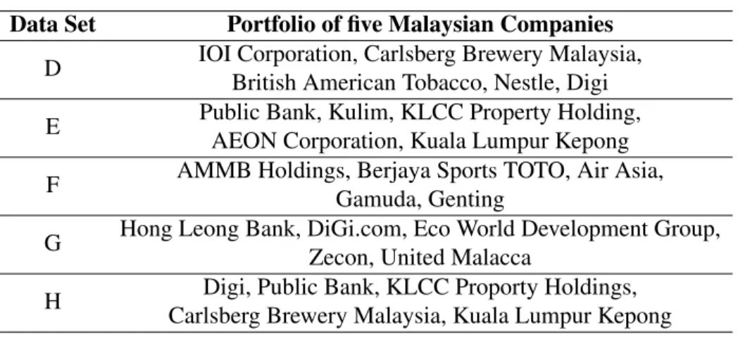
The stock data sets D, E, F, G and H were collected and compiled by previous researchers. These stock data sets consists of stocks of the Malaysian companies that are traded from 1^st March 2006 until 2^nd August 2012, consisting of a total of 1500 trading days. Table below gives the lists of stocks for data sets D, E, F, G and H.

Table 2.1: List of Malaysian companies in data sets D, E, F, G and H Data Set Portfolio of five Malaysian Companies

D IOI Corporation, Carlsberg Brewery Malaysia, British American Tobacco, Nestle, Digi E Public Bank, Kulim, KLCC Property Holding,

AEON Corporation, Kuala Lumpur Kepong F AMMB Holdings, Berjaya Sports TOTO, Air Asia,

Gamuda, Genting

G Hong Leong Bank, DiGi.com, Eco World Development Group, Zecon, United Malacca

H Digi, Public Bank, KLCC Proporty Holdings, Carlsberg Brewery Malaysia, Kuala Lumpur Kepong

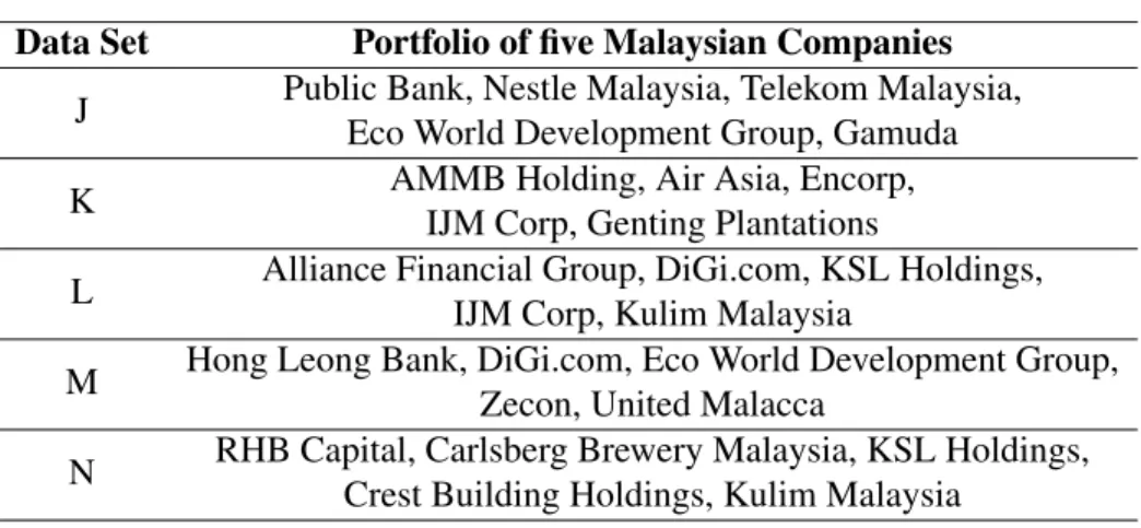
We collect and compile another 5 different stock data sets which the data collected from different stocks of the Malaysian companies that are traded from 3^rdJanuary 2005 until 4^thSeptember 2015. These data consisting a total of 2500 trading days. Table below provides the lists of stocks for data sets J, K, L, M and

N.

Table 2.2: List of Malaysian companies in data sets J, K, L, M and N Data Set Portfolio of five Malaysian Companies

J Public Bank, Nestle Malaysia, Telekom Malaysia, Eco World Development Group, Gamuda

K AMMB Holding, Air Asia, Encorp,

IJM Corp, Genting Plantations

L Alliance Financial Group, DiGi.com, KSL Holdings, IJM Corp, Kulim Malaysia

M Hong Leong Bank, DiGi.com, Eco World Development Group, Zecon, United Malacca

N RHB Capital, Carlsberg Brewery Malaysia, KSL Holdings, Crest Building Holdings, Kulim Malaysia

CHAPTER 3

UNIVERSAL PORTFOLIO GENERATED BY ZERO-GRADIENT SET OF LOGARITHM OBJECTIVE FUNCTION

3.1 Reciprocal-Price-Relative (RPR) Universal Portfolio

In this session, we introduce an additive-update universal portfolio where the updates depend on reciprocal functions of price relatives. Hence, they will be called RPR (Reciprocal-Price-Relative) universal portfolios. We will be using the objective function (1.4), which was introduced by Helmbold et al. (1998).

The gradient vector of this objective function ˆF(b_n+1) is defined as:

∇F = _∂b^∂Fˆ

n+1,i

. Then the portfolio componentsb_n+1,i,···,b_n+1,m are treated as free variables subject to the constraint ∑^m_i=1b_n+1,i = 1, with Lagrange multiplier, λ. ˆF(bn+1,λ;bn,xn)is a function of bn+1 and λ givenbn and xn. The zero-gradient set of ˆF(b_n+1,λ)is the set of{b_n+1:∇Fˆ(b_n+1,λ) =0}.

The pseudo Lagrange multiplier λ is a function of the variable b_n+1 obtained by some mathematical operation on the zero-gradient equations of the objective function 1.4. Since it is a variable, it is not a valid solution of the zero-gradient equations. The pseudo λ is said to be a pseudo solution of the zero-gradient equations.

The quantity log(b^t_n+1x_n+1) is the rate of growth of wealth on day n+1 which can be estimated by log(b^t_n+1x_n) since x_N is unknown on day n. We obtain the Type 1 RPR universal portfolio by approximating log(b^t_n+1xn)with

first-order Taylor series

log(b^t_nxn) + ^btn+1_btnx^xnⁿ−1

−1

.

3.1.1 Type 1 RPR Universal Portfolio

In this section, the derivation for Type 1 RPR universal portfolio is shown. The empirical results for this universal portfolio are given by running this universal portfolio on the stock data sets.

Proposition 3.1.1: ConsiderC= (c_{i j})be a non-negative matrix satisfying1^tC= 1where1= (1,1,···,1)andα≥0 are given. Givenξ >0, from (1.4), consider the objective function

F(bˆ n+1,λ) =ξ

log(b^t_nxn) + b^t_n+1xn

b^t_nx_n −1

−log _m

∏

i=1

[ηi+ (bn+1,i−bni)]

+λ _m

i=1

∑

bn+1,i−1

(3.1)

where

v_i= [α(b^t_nx_n) +x_ni]⁻¹ (3.2) fori=1,2,···,mand

ηi=ξ⁻¹(b^t_nx_n)

∑

m j=1

c_{i j}v_j (3.3)

fori=1,2,···,m. Then we can obtain the pseudo Type 1 RPR universal portfolio generated by the zero-gradient set of ˆF(b_n+1,λ)as followed

bn+1=bn+ξ⁻¹(b^t_nxn)[v−Cv] (3.4)

fori=1,2,···,m, whereξ is any positive scalar satisfyingb_n+1≥0.

Proof.We differentiate (3.1) with respect tobn+1,ito obtain

∂Fˆ

∂bn+1,i =ξ xni

b^t_nxn− 1

[ηi+ (bn+1,i−bni)]+λ (3.5)

fori=1,2,···,m. Then, we let (3.5) equal to 0 and rearrange the equation, we obtain

ξ xni

b^t_nxn+λ

[ηi+ (b_n+1,i−b_ni)] =1 (3.6)

fori=1,2,···,m. Then, we multiply (3.5) byb_niand sum overito get

λ =

∑

m i=1

b_ni

[ηi+ (b_n+1,i−b_ni)]−ξ. (3.7)

The variable λ that we obtained in (3.7) is known as a pseudo Lagrange multiplier. Next, we substitute this variableλ into (3.6) to obtain

ξ x_ni b^t_nx_n+

∑

m j=1

bn j

ηj+ (b_n+1,j−b_{n j})−ξ

[ηi+ (bn+1,i−bni)] =1 (3.8)

fori=1,2,···,m. Let

zi= [ηi+ (bn+1,i−bni)]⁻¹ (3.9)

fori=1,2,···,mand then (3.8) becomes

∑

m j=1

b_{n j}z_j−z_i=ξ

1− xni

b^t_nxn

(3.10)

Then, we rewrite (3.10) in matrix form,Az=ywhere

yi=ξ

1− x_ni b^t_nx_n

(3.11)

fori=1,2,···,mandA= (a_{i j})is defined as following

a_ii=b_ni−1 for i=1,2,···,m a_{i j}=b_{n j} for i6= j.

(3.12)

Then, the solution toAz=yisz=ζ1−y whereζ is any real scalar (see (3.1.1)). Hence, we have

zi=(ζ−ξ)(b^t_nx_n) +ξxni

b^t_nx_n (3.13)

fori=1,2,···,m. Then, we reparametrizeζ = (α+1)ξ and obtain

z⁻_i ¹= b^t_nxn

ξ[α(b^t_nxn+xni)] (3.14) for i=1,2,···,m. Lastly, we merge the equations (3.2), (3.3) and (3.9) and obtain

bn+1,i=bni+z⁻¹_i −ηi

=bni+ξ⁻¹(b^t_nxn)

vi−

∑

m j=1

ci jvj

(3.15)

where (3.4) is obtained.

Lemma 3.1.1: LetAbe them×mmatrix defined by (3.12).

1. The solution ofAz=ywhereydefined by (3.11) isz=ζ1−yfor any real scalarζ.

2. The solution toAq=swhereqis defined by

q_i=φ(b_n,x_n)

1− xni

b^t_nxn

(3.16)

fori=1,2,···,mand

φ(bn,xn) =ξ 1+

b^t_nx_n−(s⁻¹)^tx_n b^t_nx_n

(3.17)

iss=γ1−qfor any real scalarγ wheres⁻¹= (s⁻_i ¹).

Proof.

1. Anyz of the formz=η1−ysatisfies Az=η(A1)−Ay=ζ(A1)− (−y) =y. Conversely, ifzis a solution toAz=y, thenAz= (b^t_nz)1− z=y, implying thatz=ζ1−ywhereζ =b^t_nz_n.

2. First note thatAq= (b^t_nq)1−q=−q sinceb^t_nq=φ(b_n,x_n)∑^m_i=1 b_ni−

bnixni

b^t_nxn

=0. Anysof the forms=γ1−qwill satisfyAs=γ(A1)−Aq= q. Conversely, any solutionstoAs=qmust satisfyAs= (b^t_ns)1−s=q, implying thats=γ1−qwhereγ=b^ts.

By selecting the matrixCas

C=















0.24 0.20 0.23 0.31 0.21 0.17 0.20 0.33 0.22 0.11 0.30 0.27 0.30 0.03 0.24 0.00 0.04 0.02 0.15 0.31 0.29 0.29 0.13 0.29 0.13















(3.18)

where the sum of the entry in each of the column must be one. The matrixC above is generated randomly which ensure matrix C is a non-negative matrix which satisfy1^tC=1where1= (1,1,···,1). A 5×5 matrix is chosen because the stock data sets each consists five stocks.

Then, we run this Type 1 RPR Universal Portfolio on the stock data sets listed in Table 2.1 to obtain empirical results. The period of trading of the stocks selected in Table 2.1 is from 1^stMarch 2006 until 2^ndAugust 2012, consisting of 1500 trading days. There are five company stocks in each data set. We start with taking the initial starting portfoliob₁= (0.2,0.2,0.2,0.2,0.2)for all stock data sets. For each stock data sets, the wealthS₁₅₀₀ obtained and the final portfolios b₁₅₀₁ are calculated for the values ofα and best values of ζ are listed in Table 3.1, 3.2, 3.3, 3.4 and 3.5.

Table 3.1: The wealthS1500and the final portfoliob₁₅₀₁ achieved by the Type 1 RPR universal portfolio for stock data set D after 1500 trading days, where the initial portfoliob₁= (0.2,0.2,0.2,0.2,0.2)

α ζ S₁₅₀₀ b₁₅₀₁

0 0.00072 2.39 (0.00245, 0.16739, 0.05745, 0.71236, 0.06035) 1 0.00145 2.39 (0.00098, 0.16713, 0.05647, 0.71589, 0.05953) 2 0.00218 2.39 (0.00051, 0.16703, 0.05613, 0.71707, 0.05926) 3 0.00291 2.39 (0.00027, 0.16698, 0.05596, 0.71766, 0.05913) 4 0.00364 2.39 (0.00013, 0.16696, 0.05586, 0.71801, 0.05904) 5 0.00437 2.39 (0.00005, 0.16694, 0.05579, 0.71823, 0.05899) 6 0.00509 2.39 (0.00035, 0.16699, 0.05603, 0.71740, 0.05923) 7 0.00582 2.39 (0.00027, 0.16696, 0.05596, 0.71765, 0.05916) 8 0.00655 2.39 (0.00020, 0.16695, 0.05590, 0.71784, 0.05911) 9 0.00728 2.39 (0.00013, 0.16695, 0.05585, 0.71800, 0.05907) 10 0.00801 2.39 (0.00008, 0.16693, 0.05582, 0.71813, 0.05904)

Table 3.2: The wealthS1500and the final portfoliob1501 achieved by the Type 1 RPR universal portfolio for stock data set E after 1500 trading days, where the initial portfoliob₁= (0.2,0.2,0.2,0.2,0.2)

α ζ S₁₅₀₀ b₁₅₀₁

0 0.00072 10.29 (0.00288, 0.16725, 0.05285, 0.71626, 0.06076) 1 0.00145 10.30 (0.00111, 0.16701, 0.05631, 0.71585, 0.05972) 2 0.00218 10.31 (0.00060, 0.16695, 0.05602, 0.71704, 0.05939) 3 0.00291 10.31 (0.00034, 0.16692, 0.05588, 0.71764, 0.05922) 4 0.00364 10.31 (0.00020, 0.16690, 0.05579, 0.71799, 0.05912) 5 0.00437 10.31 (0.00009, 0.16689, 0.05574, 0.71823, 0.05905) 6 0.00509 10.31 (0.00003, 0.16688, 0.05569, 0.71840, 0.05900) 7 0.00582 10.31 (0.00031, 0.16693, 0.05591, 0.71764, 0.05921) 8 0.00655 10.31 (0.00023, 0.16692, 0.05586, 0.71784, 0.05915) 9 0.00728 10.31 (0.00016, 0.16692, 0.05582, 0.71799, 0.05911) 10 0.00801 10.31 (0.00011, 0.16691, 0.05578, 0.71812, 0.05908)

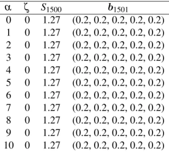
Table 3.3: The wealthS1500and the final portfoliob₁₅₀₁ achieved by the Type 1 RPR universal portfolio for stock data set F after 1500 trading days, where the initial portfoliob₁= (0.2,0.2,0.2,0.2,0.2)

α ζ S₁₅₀₀ b₁₅₀₁

0 0 1.27 (0.2, 0.2, 0.2, 0.2, 0.2) 1 0 1.27 (0.2, 0.2, 0.2, 0.2, 0.2) 2 0 1.27 (0.2, 0.2, 0.2, 0.2, 0.2) 3 0 1.27 (0.2, 0.2, 0.2, 0.2, 0.2) 4 0 1.27 (0.2, 0.2, 0.2, 0.2, 0.2) 5 0 1.27 (0.2, 0.2, 0.2, 0.2, 0.2) 6 0 1.27 (0.2, 0.2, 0.2, 0.2, 0.2) 7 0 1.27 (0.2, 0.2, 0.2, 0.2, 0.2) 8 0 1.27 (0.2, 0.2, 0.2, 0.2, 0.2) 9 0 1.27 (0.2, 0.2, 0.2, 0.2, 0.2) 10 0 1.27 (0.2, 0.2, 0.2, 0.2, 0.2)

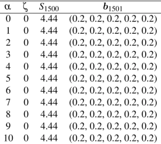
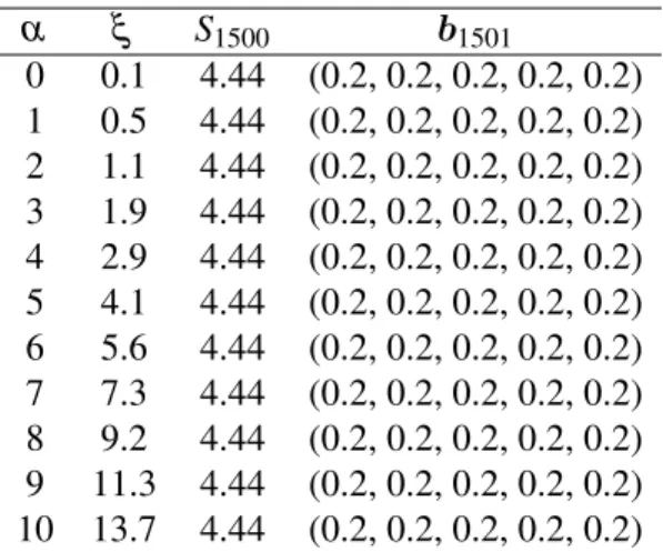
Table 3.4: The wealthS1500and the final portfoliob1501 achieved by the Type 1 RPR universal portfolio for stock data set G after 1500 trading days, where the initial portfoliob₁= (0.2,0.2,0.2,0.2,0.2)

α ζ S₁₅₀₀ b₁₅₀₁

0 0 4.44 (0.2, 0.2, 0.2, 0.2, 0.2) 1 0 4.44 (0.2, 0.2, 0.2, 0.2, 0.2) 2 0 4.44 (0.2, 0.2, 0.2, 0.2, 0.2) 3 0 4.44 (0.2, 0.2, 0.2, 0.2, 0.2) 4 0 4.44 (0.2, 0.2, 0.2, 0.2, 0.2) 5 0 4.44 (0.2, 0.2, 0.2, 0.2, 0.2) 6 0 4.44 (0.2, 0.2, 0.2, 0.2, 0.2) 7 0 4.44 (0.2, 0.2, 0.2, 0.2, 0.2) 8 0 4.44 (0.2, 0.2, 0.2, 0.2, 0.2) 9 0 4.44 (0.2, 0.2, 0.2, 0.2, 0.2) 10 0 4.44 (0.2, 0.2, 0.2, 0.2, 0.2)

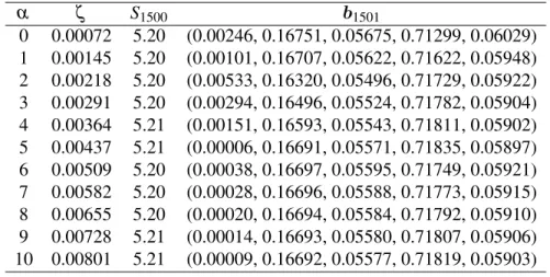
Table 3.5: The wealthS1500and the final portfoliob₁₅₀₁ achieved by the Type 1 RPR universal portfolio for stock data set H after 1500 trading days, where the initial portfoliob₁= (0.2,0.2,0.2,0.2,0.2)

α ζ S₁₅₀₀ b₁₅₀₁

0 0.00072 5.20 (0.00246, 0.16751, 0.05675, 0.71299, 0.06029) 1 0.00145 5.20 (0.00101, 0.16707, 0.05622, 0.71622, 0.05948) 2 0.00218 5.20 (0.00533, 0.16320, 0.05496, 0.71729, 0.05922) 3 0.00291 5.20 (0.00294, 0.16496, 0.05524, 0.71782, 0.05904) 4 0.00364 5.21 (0.00151, 0.16593, 0.05543, 0.71811, 0.05902) 5 0.00437 5.21 (0.00006, 0.16691, 0.05571, 0.71835, 0.05897) 6 0.00509 5.20 (0.00038, 0.16697, 0.05595, 0.71749, 0.05921) 7 0.00582 5.20 (0.00028, 0.16696, 0.05588, 0.71773, 0.05915) 8 0.00655 5.20 (0.00020, 0.16694, 0.05584, 0.71792, 0.05910) 9 0.00728 5.21 (0.00014, 0.16693, 0.05580, 0.71807, 0.05906) 10 0.00801 5.21 (0.00009, 0.16692, 0.05577, 0.71819, 0.05903)

Table 3.1, 3.2, 3.3, 3.4 and 3.5 give the empirical performance of Type 1 RPR universal portfolio. We can observed that the best wealth of 10.31 units is obtained for data set E corresponding toα=6 andζ =0.0051. The lowest wealth of 1.27 units is obtained for data set F corresponding toα=0,···,10 and ζ =0. Average wealth of 2.39, 4.44 and 5.20 units are obtained for data set D, G and H respectively. It is also observed that for data sets D, E, and H, a proportion of 70% of the current wealth after 1500 trading days tends to be invested in the fourth company of the portfolio, whereas the proportion invested in the first company tends to zero. This indicates that the fourth and the first stocks are the best and worst stock respectively. For data sets F and G, the portfolios become constant after a long run.

3.1.2 Type 2 RPR Universal Portfolio

In this section, the derivation for Type 2 RPR universal portfolio is shown. The empirical results for this universal portfolio are given by running this universal portfolio on the stock data sets.

Proposition 3.1.2: ConsiderC= (c_{i j})be a non-negative matrix satisfying1^tC= 1where a real scalar,αare given. Givenξ>0, from (1.4), consider the objective function

F(bˆ _n+1,λ) =ξ

log(b^t_nx_n) +

b^t_n+1x_n b^t_nxn

−1 2

b^t_n+1x_n b^t_nxn −1

2

−log _m

∏

i=1[σi+ (b_n+1,i−bni)]

+λ _m

i=1

∑

b_n+1,i−1

(3.19)

where

σi=ξ⁻¹(b^t_nxn)²

∑

m j=1

ci jrj (3.20)

fori=1,2,···,m,

r_i=

α(b^t_nx_n)²+ x_ni−β(b_n,x_n)

(b^t_nx_n) +β(b_n,x_n)x_ni−1

>0 (3.21)

fori=1,2,···,mand

β(bn,xn) =ξ⁻¹(b^t_nxn)²x^t_n[Cr−r]. (3.22)

Then, the pseudo Type 2 RPR universal portfolio generated by the zero-gradient set of ˆF(b_n+1,λ)is obtained as follow

bn+1=bn+ξ⁻¹(b^t_nxn)²[r−Cr] (3.23)

forn=1,2,···, whereξ is any positive scalar satisfyingb_n+1≥0, providedris

a consistent solution of (3.21).

Proof. Then, we differentiate ˆF(b_n+1,λ)in (3.19) with respect tob_n+1,ito obtain

∂Fˆ

∂b_n+1,i=ξ2x_ni

b^t_nx_n−(b^t_n+1xn)xni

(b^t_nx_n)²

−[σi(bn+1,i−bni)]⁻¹+λ (3.24)

fori=1,2,···,m. Then we let _∂b^∂Fˆ

n+1,i in (3.24) to be zero and obtain ξ2x_ni

b^t_nx_n−(b^t_n+1xn)xni

(b^t_nx_n)²

−[σi+ (bn+1,i−bni)]⁻¹+λ =0 (3.25)

fori=1,2,···,m. Next, we multiply (3.25) byb_niand sum overito obtain the pseudo Lagrange multiplier

λ =−ξ

2−b^t_n+1xn

b^t_nx_n

+

∑

m j=1

bn j σj+ (bn+1,j−bn j)₋1

. (3.26)

Then, we substitute the Lagrange multiplier in (3.26) into (3.25) to get

ξ2xni

b^t_nxn−(b^t_n+1x_n)x_ni

(b^t_nxn)² −2+b^t_n+1x_n b^t_nxn

−[σi+ (b_n+1,i−b_ni)]⁻¹] +

∑

m j=1

bn j σj+ (b_n+1,j−bn j)₋1

=0

(3.27)

fori=1,2,···,m. Then, we let

s⁻_i ¹=b_ni−b_i+σi (3.28)

fori=1,2,···,m. Then, we substitute (3.28) into (3.27) to obtain

∑

m j=1

bn jsj−si=φ(bn,xn)

1− x_ni b^t_nx_n

(3.29)

fori=1,2,···,mwhere

φ(bn,xn) =ξ

2−b^t_n+1x_n b^t_nx_n

. (3.30)

We use the vector notation s⁻¹ = (s⁻_i ¹) then (3.28) can become (s⁻¹)^tx_n = b^t_n+1xn−b^t_nxn+σ^txn. This implies

b^t_n+1xn

b^t_nx_n =1+(s⁻¹)x_n−σ^tx_n

b^t_nx_n . (3.31)

By substituting (3.31) into (3.30), we obtain the equivalent definition of φ(bn,xn)in (3.17). The matrix form of the set of equations on (3.29) isAs=q where A and q are defined by (3.12) and (3.16) respectively. From Lemma (3.1.1), we have shown that the solution toAs=q is s=γ1−q for any real scalarγ. An equivalent definition ofβ(b_n,x_n)in (3.22) is given by

β(bn,xn) = (x^t_nσ−x^t_ns⁻¹). (3.32)

Hence, we can obtainsi=γ−qi=γ−ξ[1+^β(b_bt^n,xn)

nxn ]fori=1,2,···,mfrom (3.16), (3.17) and (3.32).

Then we reparametrize theγas(α+1)ξ, we obtain

s_i=(bnx)⁻²ξ[α(b^t_nx_n)²+ (x_ni−β(b_n,x_n))(b^t_nx_n) +β(b_n,x_n)x_ni]

=(b^t_nx_n)⁻²r⁻_i ¹

(3.33)

for i=1,2,···,m where r_i is defined by (3.21). From (3.20) and (3.28), we obtain the next-day portfolio

b_n+1,i=b_ni+s⁻_i ¹−σi

=b_ni+ξ⁻¹(b^t_nx_n)²

r_i−

∑

m j=1

c_{i j}r_j

(3.34)

fori=1,2,···,mand (3.23) is proved.

We remark that the pseudo Type 2 RPR universal portfolio may be relaxed by assuming thatβ(b_n,x_n)is a constant, which not depending on theb_nandx_n. The pseudo relaxed type 2 portfolio has parametric set(C,α,β)where we will

choose the β to be−1≤β ≤1. The scalar α is chosen so that r_i>0 for all i=1,2,···,min (3.21). This is always possible for a large enoughα.

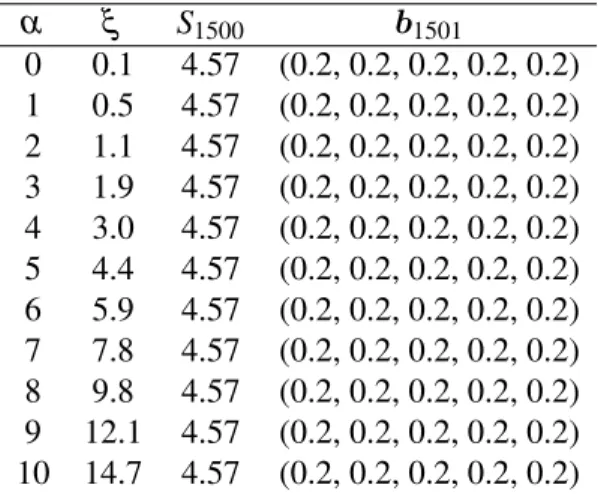
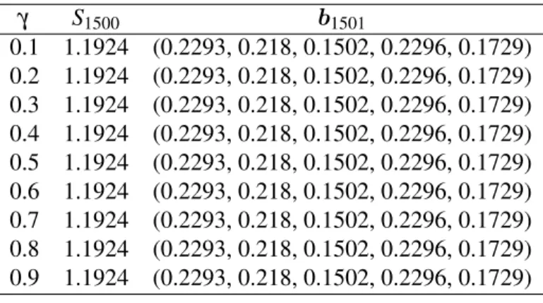
Similarly, we run the pseudo relaxed Type 2 RPR universal portfolios with parametric set(C,α,β)on the stock data sets D, E, F, G and H, listed in Table 2.1. We select the matrixCto be an equal-entry matrix with each entry 0.2 and eleven integer values of α from 0 until 10. β =0.6 is selected to obtain the empirical results. The best wealth S₁₅₀₀ achieved after 1500 trading days on each stock data sets are listed in Table 3.6, 3.7, 3.8, 3.9 and 3.10.

Table 3.6: The wealthS₁₅₀₀ and the final portfoliob₁₅₀₁achieved by the pseudo relaxed Type 2 RPR universal portfolio for stock data set D after 1500 trading days, where the initial portfoliob1= (0.2,0.2,0.2,0.2,0.2)

α ξ S₁₅₀₀ b₁₅₀₁

0 0.1 2.46 (0.24380, 0.21627, 0.21218, 0.17654, 0.15121) 1 0.5 2.53 (0.23456, 0.23665, 0.22449, 0.17672, 0.12758) 2 1.3 2.57 (0.23182, 0.25012, 0.23215, 0.17530, 0.11061) 3 2.2 2.57 (0.22625, 0.25142, 0.23250, 0.17754, 0.11229) 4 3.5 2.58 (0.22423, 0.25482, 0.23428, 0.17777, 0.10890) 5 5.1 2.59 (0.22281, 0.25718, 0.23550, 0.17794, 0.10657) 6 6.9 2.59 (0.22144, 0.25796, 0.23587, 0.17839, 0.10634) 7 9.0 2.59 (0.22048, 0.25876, 0.23626, 0.17865, 0.10585) 8 11.4 2.59 (0.21978, 0.25950, 0.23663, 0.17881, 0.10528) 9 14.0 2.59 (0.21909, 0.25969, 0.23671, 0.17906, 0.10545) 10 16.9 2.59 (0.21857, 0.25998, 0.23684, 0.17923, 0.10538)