This project deals with the Bézier method in computer aided geometric design (CAGD) which involves Bézier Curve and Bézier Surface which is widely related to the other theorem and method. The aim of this project is to introduce the basic of Bézier method and then generate the Bézier curves, Bézier surfaces, theory and properties and develop Bézier method in image processing application specifically image compression using MATLAB. The Bézier method has been widely applied in many fields, especially in computer-aided geometric design (CAGD), but there are only several applications in image processing.
This project will focus on Bézier Curve, Bézier Surface, Bernstein Polynomial, de Casteljau Algorithm, Interpolation, Approximation, Quad Tree and Parametric Line Fitting, Image Rescaling and Image Compression. For the main focus of this project which is image compression with RGB Quadtree Decomposition and Parametric Line Fitting method, the analysis is done for four different images which are Peppers.tiff, Baboon.tiff, Airplane.tiff and Lena.png. I would like to take this opportunity to express my deepest gratitude to all parties involved in the realization of this project, starting from the lecturers of UTP, my friends and family who have helped me in the realization of the project.
Last but not least, thanks also go to others whose names were not mentioned on this page, but who in one way or another contributed to the realization of this project. 83 Figure 113: Threshold versus RMSE and PSNR combination for Peppers.tiff 94 Figure 114: Threshold versus RMSE and PSNR combination for Baboon.tiff 94 Figure 115: Threshold versus RMSE and PSNR combination for Airplane.tiff 95 Figure 116: Combination of Threshold vs. RMSE & PSNR for Lena.png 95.
INTRODUCTION
- Background of Study
- Problem Statement
- Objectives
- Scope of Study
Two of the most important mathematical representations of curves and surfaces in computer graphics and computer-aided design are Bézier and B-spline shapes. Their popularity is due to the fact that they have many mathematical properties that allow them to be manipulated and analyzed, yet the use of curves does not require mathematical knowledge [3]. The Bézier method has been widely used in many fields, especially in computer-aided geometric design (CAGD).
The Bézier curves and surfaces were famously used in design problems and play an important role in the construction of completely different products such as car bodies, ship hulls, propeller blades, shoes and bottles, and even in the description of geological, physical and medical phenomena. In order to vary the techniques in image processing and perhaps improve the available techniques, the author will try to implement the Bézier method for image processing specifically image compression. To implement the Bézier method for image processing specifically image compression and simulation of theory and properties.
It will cover the theory and properties of Bernstein polynomial, de Casteljau algorithm, spline, Bézier curves, Bézier surfaces, image processing application such as affine transforms, image rescaling, image reconstruction and image compression. The author will try to implement Bézier method for image processing including cubic interpolation, least square fitting and bilinear interpolation.
LITERATURE REVIEW
Bézier Curve
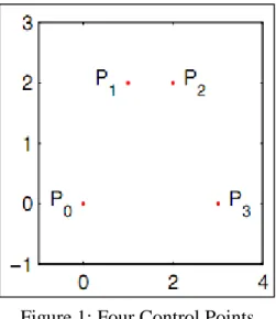
- Linear Bézier Curves
- Quadratic Bézier Curves
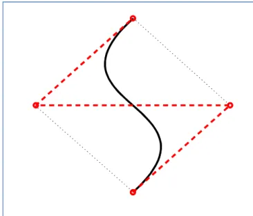
- Cubic Bézier Curves
- Deriving the Curve
- Subdivisions and Generating New Control Points 11
- Properties of Bézier Curves
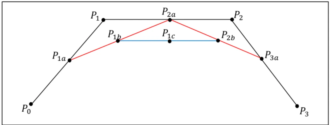
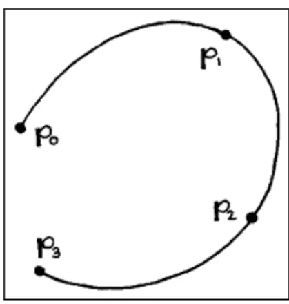
The matrix representation of the Bernstein polynomial allows multiple values to be entered quickly and calculated using a computer to generate points on the Bézier curve. The easiest way to do this is to subdivide the curve into parts and find new control points for each of the subdivisions. To do this, take the matrix form of the Bernstein polynomial equation (2.14) and then decide which part of the curve needs to be changed.
If we take the first part of the reparameterization (), +(-), which is the first half of (), and write it in matrix form, we can determine the control points of the matrix. To find these points, we need to multiply the vector of 9 points by a ratio of 3. We can do this same process for +(+-) to create a 3(,/) matrix that we can use to find a new control point for the other half of the curve.
This works for any subdivision of the original matrix and allows us to find the new control points for the subdivision. The convex hull of the control points is often called the convex hull of the Bézier curve.
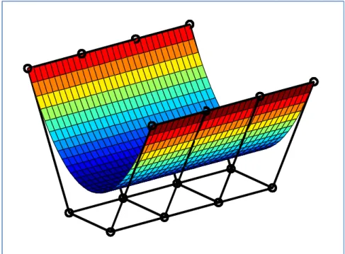
Bézier Surface
- Bilinear Bézier Surfaces
- Biquadratic Bézier Surfaces
- Bicubic Bézier Surfaces
- Properties of Bézier Surfaces
This algorithm can also be used to split a single Bézier curve into two Bézier curves at an arbitrary parameter value. The de Casteljau algorithm provides a method to evaluate the point on a Bézier curve corresponding to the parameter value ∈ [0,1]. For the case of a cubic Bézier curve with control points , , , and , and for a specified parameter value ∈ [0,1], the de Casteljau algorithm is expressed by the recursive formula.
Each point on a Bézier curve has a parameter value; to solve our problem we need to assign a parameter value W to each W . This simply states that we want the Bézier curve to pass through the data points at the correct parameter values. For data to be fitted by cubic Bézier, the first and last control points of Bézier curve are first and last point of the input data segment.
The input data can be divided into multiple segments or only one segment by specifying the initial breakpoint set, but the intermediate and cubic Bézier control points must be defined. After defining the control points, Bézier curves can be fitted to a large number of original data points with very few control points using Bézier interpolation. The output data consists of quadratic Bézier control points and the difference between the original and fitted data.
To understand how the quadratic Bézier curve can be used to fit video data, we need to understand the nature of video. An important factor when fitting data via the quadratic Bézier curve is finding the fewest number of control points [20]. This less entropy of output data is mainly due to the fact that the quadratic Bézier curve approximates the original video data with a fairly good level of accuracy.
This type of application uses Bézier curve representations for effective fingerprint image compression. In the proposed scheme, each ridge is visualized as a cubic Bézier curve and Bézier control points are determined. So any fingerprint image with n ridges can be compressed into a file containing 4*n Bézier control points.
It is sufficient to save all four Bézier control points instead of saving the actual Bézier curve (ridge). The original ridge can be reproduced from these saved control points using the properties of Bézier curve.
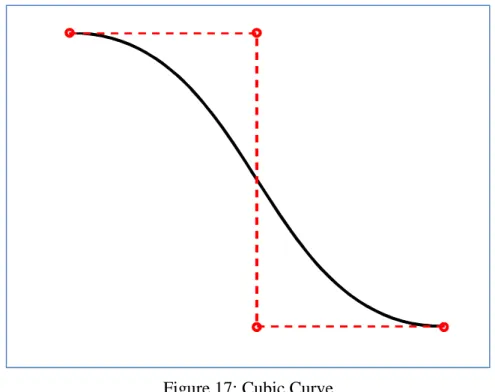
Cubic Bézier Curve with two inflection points . 50
Cubic Bézier Curve with cusp
Variation Diminishing Property
Combination of Bézier Curve
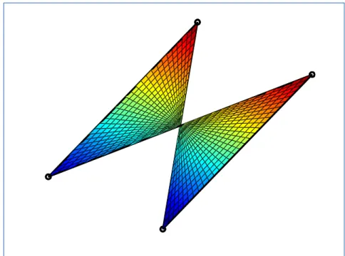
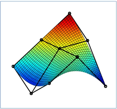
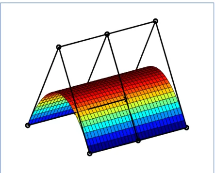
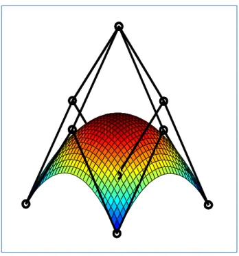
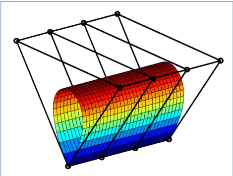
Combination of Bézier Surface
Utah Teapot
Cubic Interpolation
Image Rescaling Using Bilinear Interpolation
Bézier Curve Least Square Fitting
RGB Quadtree Decomposition and Parametric
- Uniform Threshold Variation
- Non-uniform Threshold Variation
From the quantitative analysis in two tables above, we can see the comparison of value for MSE, RMSE and PSNR for each RGB channel and also file size for original and decoded images. From the above value, we can observe the best result by looking at lowest MSE and RMSE value and highest PSNR value. The lowest MSE and RMSE and highest PSNR determine the best quality of image compression.
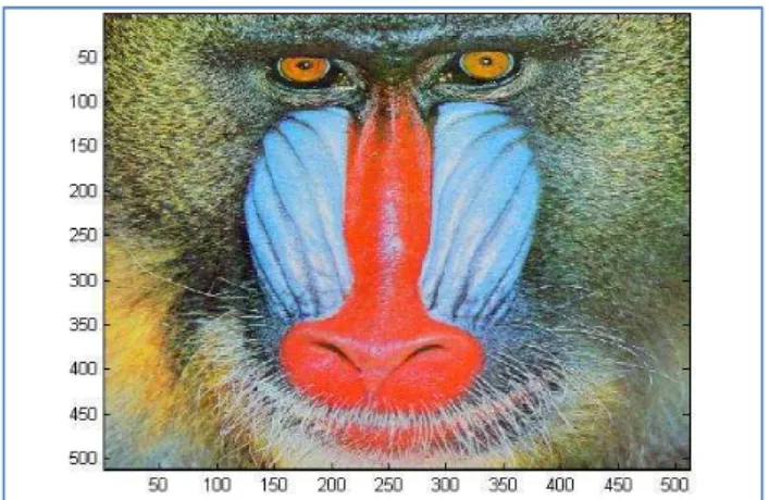
From the four images tested, we can see that the best result is Baboon.tiff and if we observe the image itself, we can see that the quality is better than the others. We then analyze the comparison between the threshold and the average MSE for each image; Peppers.tiff, Baboon.tiff, Airplane.tiff and Lena.png. The average MSE is arranged in descending order so that we can see which color channel belongs to the highest threshold.
For Baboon.tiff, the blue channel contributes the most error when its threshold value is highest. From the analyzes performed for uneven threshold variations, we can also determine the best combination of uneven thresholds. Average RMSE and PSNR values were calculated to determine the best uneven threshold combination.
From the quantitative analysis, the quality of images is determined by the lowest values of MSE and RMSE and highest value of PSNR. The graph of threshold combination versus RMSE & PSNR is plotted as on the next page. From the plotted graph on the previous pages, for the Peppers.tiff image, from Figure 113, we can see that the threshold combination that achieves the lowest RMSE and highest PSNR is the ninth combination, which is.
For the Baboon.tiff image, from Figure 114, we can see the threshold combination that achieves the lowest RMSE and PSNR is the eighth combination, which is. For the Airplane.tiff image, from Figure 115, we can see the threshold combination that achieves the lowest RMSE and PSNR is the ninth combination, which is. For the Lena.png image, from Figure 116, we can see the threshold combination that achieves the lowest RMSE and PSNR is the ninth combination, which is.
For the RGB Quadtree Decomposition and Parametric Line Matching method for image compression, from the analysis and output images of variation threshold in uniform and non-uniform patterns, we can see the quality of image Baboon.tiff is better than others even all the Red, Green and Blue channels are at a high threshold. The reason is that we can see the pure colors of the image Baboon.tiff itself which contains all the RGB color components.
CONCLUSION AND RECOMMENDATION
Conclusion
Recommendation
8] http://en.wikipedia.org/wiki/Bernstein_polynomial [9] http://en.wikipedia.org/wiki/De_Casteljau's_algorithm [10] http://en.wikipedia.org/wiki/Spline_( mathematics) [11] http://en.wikipedia.org/wiki/Image_processing. Khan, Using Spline and Quadtree for Lossy Temporal Video Data and Lossless Compression of Synthetic Image Data, Keio University. In the following figures we can see the change of the Bézier curve by changing the control points.