1
Ch 3. New Trade Theory :
(1980-2000)Core and Periphery Model
1 Introduction
I. Concerning Problem
How do the interactions among increasing returns at the level of the firm, transport costs, and factor
mobility can cause spatial economic structure to merge and change?
2
II. Finding
When transportation costs (or, more generally, trade costs) are sufficiently low, Krugman (1991) has shown that all manufactures are concentrated in a single region that becomes the “Core” of the economy, whereas the other region, called the
“Periphery”, supplies only the agricultural good.
For exactly the opposite reason, the
economy displays a symmetric regional pattern of production when transportation costs are high enough.
3
III. Market Equilibrium
The finding of market equilibrium by Krugman (1991) is the outcome of the interplay between a dispersion force and an agglomerate force.
References:
1. Krugman, P.R. (1991), “Increasing returns and
economic geography”, Journal of Political Economy 99, 483-499.
2. Fujita, M., P.R. Krugman, and J. V. Anthony (1999), The Spatial Economy, Ch.5, The MIT Press.
4
(i)
The Centrifugal force
(1) the spatial immobility of farmers (or the unskilled labors) whose demands for the manufactured good are to be met.
(2) The increasing competition that arises when firms are more agglomerated.
Market-crowding effect: Baldwin et al.
(2003).
5
Market-crowding effect:
The firms increase the competition for customers in the region with more firms, and reduce it in the region with less firms.
It implies that the firms in the region with more firms will pay a lower nominal wage in order to break even, while the opposite happens in the region with less firms.
6
(ii) The Centripetal force
(1) First, if a larger number of manufactures are located in one region, the number of varieties locally produced is also larger.
(2) Then, because firms do not price discriminate between regions, the equilibrium price index of manufactured goods is lower in this region.
7
(3)This in turn, induces some workers living in the smaller region, to move toward the large region, where they may enjoy a higher standard of living.
(4)The resulting increase in the numbers of workers creates a larger demand for the differentiate good.
(5)The increasing demand for the differentiate good leads additional firms to locate in this region.
Summary:
(1)-(3): Cost-of-living effect (Baldwin et al. 2003);
Forward linkage (Krugman, 1991).
(4)-(5): Market-access effect (Baldwin et al. 2003);
Backward linkage (Krugman, 1991).
8
Cost-of-living effect
It concerns the impact of firms’ location on the local cost of living.
The goods tend to be cheaper in the region (country) with more industrial firms since
consumers in this region (country) will import a narrower range of products and thus avoid more of trade cost.
Market-access effect
It describes the tendency of monopolistic
firms to locate their production in the big market and export to small market.
9
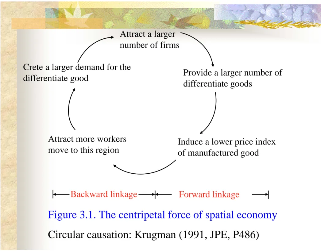
Provide a larger number of differentiate goods
Figure 3.1. The centripetal force of spatial economy Circular causation: Krugman (1991, JPE, P486)
Attract a larger number of firms Crete a larger demand for the
differentiate good
Attract more workers
move to this region Induce a lower price index of manufactured good
Forward linkage Backward linkage
10
IV. Circular causation
(i) Backward linkage
Because of economies of scale, production of
each manufactured good will take place at only a limited number of sites. Other things equal, the preferred sites will be those with relatively large nearby demand, since producing near one’s main market minimizes transportation costs. Other
locations will then served from these centrally located sites.
Manufactures production will tend to concentrate where there is a large market.
11
(ii) Forward linkage
Other things equal, it will be more desirable to live and produce near a concentration of
manufacturing production because it will then be less expensive to buy the goods this central place provides.
The market will be large where manufactures production is concentrated.
12
2. Assumptions
(1) In a spatial economy, there exists two sectors, monopolistically competitive manufacturing M and perfectly competitive agriculture A.
(2) Each of these sectors employs a single resource, workers and farmers respectively.
(3) Each of these sector-specific factors is in fixed supply.
(4) The geographical distribution of resources is
partly exogenous, partly endogenous. Let there be R regions.
13
(i) Exogenous
The world has farmers (or unskilled labors), and each region is endowed with an exogenous share of this world agricultural labor force
denoted . (ii) Endogenous
The manufacturing labor force (or skilled labors), by contrast, is mobile over time; at any point in
time we denote the share of region in the world supply by . It is convenient to choose units so that
LA
LM
, A 1
M L
L
14
(5) Agricultural goods can be freely transported, and manufactured goods are subject to “iceberg
transport cost”. That is, if one unit of a good is shipped from to s, only units arrive.
Where .
3. Derivations
Since the shipment of agricultural goods is assumed costless, and because these good are produced with constant returns, agricultural
workers have the same wage rate in all regions.
We use this wage rate as the numeraire, so .
1 Ts
1 Ts
1 wA
15
(2) Wages of manufacturing workers, however,
may differ both in nominal and in real terms. Let us, define and to be the nominal and real
wage rate, respectively, of manufacturing workers in region .
(3) Other things equal, manufacturing workers will move toward regions that offer high real wages and away from regions that offer below- average real wage.
w
16
4. The Model
(1) Income
The income of region is given by
(3.1) : The total units of manufacturing workers in the
world.
: The total units of farmers in the world.
: The share of manufacturing workers in the region , where , and
w (1 ) Y
1
0 1
R
1
1
17
: The share of farmers in the region ( = 1/R), : The nominal wage rate in the region .
w
(2) Price Index
From (2.80) and (2.84), the price index of manufactures in region is given by
(3.2)
The price index in would tend to be lower, the higher the share of manufacturing that is in regions with low
transport cost to .
1
1
)1
(
s
s s s w T G
18
From equation (3.2), suppose that wages in different regions were the same, then the price index in would tend to be lower, if the higher the share of manufacturing that is in region with low
transport costs to , .
, G
s
Ts
19
That is,
keep the same, then
s s
s ,T ,w
s(wsTs )1
)
(
1 R 1 s
s s
s w T
)
( 1-
1 1
1
R s
s s s w T
G
20
The Examples of two regions
Suppose there are only two regions in the
economy, a shift of manufacturing into one of the regions would tend, other thing equal, to lower the price index in that region – and thus make the region a more attractive place for manufacturing workers to live and work.
The effect of the forward linkages
21
Explanation:
w w
w1 2
1
, 1
, 2 12 21
1 T T T
1 1 11
1 w (1 )(wT)
G
1 1 11
2 (wT) (1 )w
G
1 1 11
1 w (1 )(wT)
G
w1 (wT)1 T1 w1 11
(1 T1 ) w1 (wT)1 11
,then
22
Since then thus
Therefore, if
,
1
T T1 1, (1T1 ) 0,
(1 T1 )w1 (wT)1
(1 T1 )w1 (wT)1 11
G1
23 From the equation (2.75) in previous chapter, we know
that the “indirect utility function” is given by
(3.4) Since we normalize , and for the
manufacturing workers, thus
(3.5) (3.6) If then
Similarly,
) 1 (
1
( )
) 1
(
Y G
P
A V
1
PA Y w w
1 (1 )1 wG1
2 (1 )1 wG2
1
G V1
2
2 V
G
24
(3) Nominal wage
(3.7)
From equation (3.7), suppose that the price indexes in all region were identical, ,
Then, the nominal wage rate in region , tends to be higher, if incomes in other regions with low transport cost from are high.
/ 1 1
1
s
s s
sT G
Y w
G
Gs s 1,2,....R.
w
25 That is,
If, and
then
, G
Gs Ys Ts
) (YsT1s
1 1
1
G
T Y
R s
s s
/ 1 1 1
1 G
T Y
R s
s s
w
It implies that firms can afford to pay higher wages if they have good access to a larger market.
The effect of the backward linkages.
26 (4) The Real Wages
From (3.4), (3.5), and (3.6), if the price of agricultural good is normalized as equal one everywhere, then we have
(3.8)
Where denotes “ the cost-of-living index” in region , Thus, we can specify “the real wage” in region as,
(3.9)
That is, the real wage is defined as “ the nominal wage be deflated by the cost-of-living index ”
(
) Y GV 1 1
G
w G
w
G
27
5. Determination of Equilibrium
From previous section, we summarize the system of equations as:
(3.10) (3.11) (3.12)
(3.13)
w (1 ) Y
1 / 1 1
1
) (
R s
s s s w T G
/ 1 1 1
1
R s s
s
sT G
Y w
w G
28
(3.14) (3.15)
Finally, in equilibrium, we need
(3.16)
Thus, if the transportation cost, , between regions r and s for all regions and ,are given, then there are 6R
equations for instantaneous equilibrium to determine 6R endogenous variables.
( ) Y G
V 1 1
1,2,...R, s s
1
1
R s
s
Ts
,
,w , ,G , and V Y
. ,...
,....
2 ,
1 s R
s
29
6. The Core-Periphery Model: the Numerical Simulation
Core-Periphery Model:
In general, the core-periphery model is the
special case of the model described above when there are only two regions and agriculture is evenly divided between those two regions. i.e.,
2 1
2 1
30
If we define the transportation cost between two region is T, and represent region 1’s share of manufacturing, then, we have
(3.17) (3.18) (3.19) (3.20)
) 1
2 ( 1
1
1 w
Y
) 1
2 ( ) 1
1
( 2
2 w
Y
11 2 1 1/1
1 [ w (1 )(w T) ]
G
1 1 12 1/1
2 [ (wT) (1 )w ] G
31 (3.21)
(3.22) (3.23) (3.24)
--- (3.25)
(3.26) (3.27)
This model has eleven simultaneous nonlinear equations to determine eleven endogenous variables:
1 1 1/
2 2 1
1 1
1 [Y G Y G T ] w
1 1/
2 2 1 1
1 1
2 [Y G T Y G ] w
1 w1G1
2 w2G2
1 1 1
1 (1 ) Y G
V
1 2 2
2 (1 ) Y G
V
2
1
, , , , ,
, , ,
,
, 2 1 2 1 2 1 2 1 2
1 Y G G w w V V
Y
32 0
2
1
0.0 0.5 1
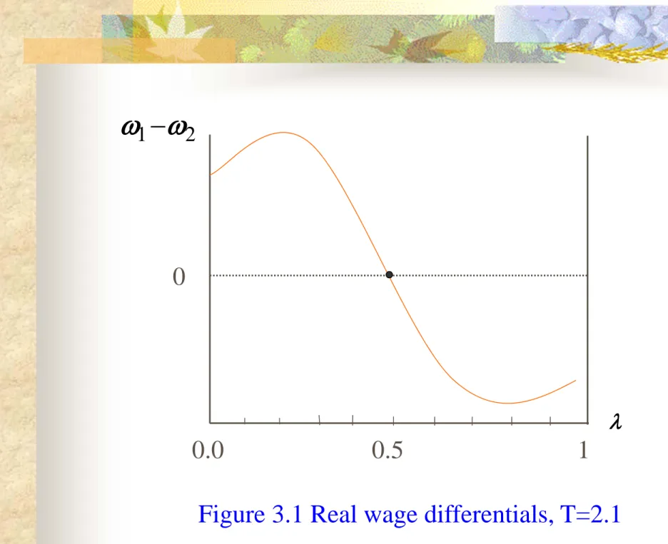
Figure 3.1 Real wage differentials, T=2.1
33
The transport cost is high enough.
The wage differential is positive if is less than , negative if is greater than .
It implies that if a region has more than half the manufacturing labor force, it is less attractive to workers than the other region.
This means that in this case the economy
converges to a long-run symmetric equilibrium in which manufacturing is equally divided between the two regions.
2
1
2 1
34 Figure 3.2 Real wage differentials, T=1.5
0
0.0 0.5 1
2
1
35
a low transport cost T.
the wage differential slopes strictly upward in .
the higher the share of manufacturing in either region, the more attractive the region becomes.
Other things equal, a larger manufacturing labor force makes a region more attractive both because the larger local market leads to higher nominal wages (backward linkage) and because the larger variety of locally produced goods
lowers the price index (forward linkage)
36
Although an equal division of manufacturing
between the two regions is still an equilibrium, it is now unstable.
If one region should have even a slightly
larger manufacturing sector, that the sector would tend to grow over time while the other region’s manufacturing shrink, leading eventually to a core-periphery pattern with all manufacturing concentrated in one region.
37 Figure 3.3 Real wage differentials, T=1.7
0
0.0 0.5 1
2
1
38
An intermediate level of transport cost
The symmetric equilibrium is locally stable,
There are two unstable equilibria flank the
symmetric equilibrium if starts from either a
sufficiently high or a sufficiently low initial value, the economy converges not to the symmetric
equilibrium but to a core-periphery pattern with all manufacturing in only one region.
This picture then has five equilibrium: three stable (the symmetric and manufacturing concentration in either region) and two unstable.
2) ( 1
39
From these three cases, Figure 3.1-Figure 3.3, it is straight forward to describe the equilibrium
pattern as shown in Figure 8.4, which shows how the types of equilibria vary with transport cost.
40 0.5
1.0 1.5
0.0 1.0
T(S) T(B)
T Figure 3.4 Core-periphery bifurcation
41
In Figure 3.4, solid lines indicate stable equilibria, broken lines unstable.
At sufficiently high transport costs, there is a
unique stable equilibrium in which manufacturing is evenly divided between the region.
When transport costs fall below some critical level, T(s), new stable equilibria emerge in which all
manufacturing is concentrated in one region.
42
When they fall below a second critical level, T(B), the symmetric equilibrium becomes unstable.
The critical level, T(s), is the point at which a
core-periphery pattern, once established, can be sustained.
The second critical level, T(B), is the point at
which symmetry between regions must be broken because the symmetric equilibrium is unstable.