Such frictions are introduced into the environment by exploiting – in several different ways – the concept of spatial/informational separation introduced by Townsend (1980). This is an equilibrium model for search and matching in the tradition from e.g. Lucas and Prescott (1974), Hellwig (1976), Diamond (1982), Mortensen (1982) or Pissarides (1990).1 The central concern of this methodology is the provision of an explicit link between the environmental constraints - especially spatial and informational - the assumed trade frictions in the environment and the possible allocations.
Two different competitive equilibrium regimes are studied: one where private money is prohibited and one where it is permitted. This effect disappears when private money is allowed, and so the optimal monetary regime is different.
Finance
Optimal financial regulation
We show that when deposit insurance premiums are low, monetizing bank bailout costs may be no more inflationary than financing these costs from general revenues. This is because, while monetizing the cost increases the inflation tax rate, higher levels of general taxation reduce savings, deposits, bank reserves and the inflation tax base.
1 Introduction
We also find that low deposit insurance premiums or low reserve requirements may not be associated with a high rate of bank failure. When deposit insurance premiums are low, both factors have roughly the same effect on equilibrium inflation.
2 The model
- Firms
- Bankers
- Depositors
- The government
In terms of deposit insurance, we assume that the government imposes a premium fixed rate of ρ ≥0 per unit deposited.10 The problem then arises of what the government does with the income from deposit insurance premiums. Formal deposit insurance, as offered in the US, allows for risk-based deposit insurance premiums.
3 Bank behavior
Strategy 1
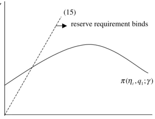
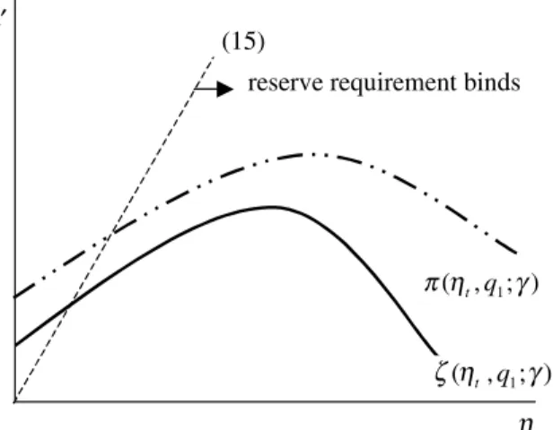
When the expected profit from the diversion of funds, in the absence of any intermediate monitoring, exceeds the expected profit from investing in project 1, then there is a moral hazard problem associated with the bank following strategy 1. And, if we define≡rt/ (1-θ −ρ), then the expected cost of bank funds according to strategy 1 takes the formq1[rt−ηt.
Strategy 2
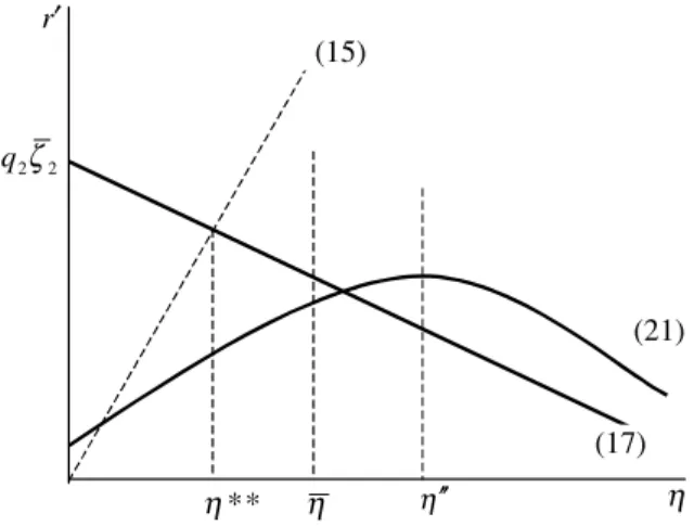
The bank's expected income under strategy 2 is its net income from loans, q2ζ¯2, plus its income from reserves, θq2Rt.
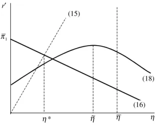
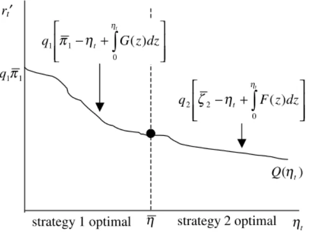
Optimal bank behavior
4 Government budget balance
- Sources equal uses of funds
- Government revenue
- Government costs
- Budget balance
The government also collects deposit insurance premiums from all active banks and reinvests the proceeds. Similarly, if banks follow strategy 2 att, they will fail with probabilityF(ηt)att+ 1, which imposes monitoring costs on the government ofγF(ηt), and the government must also cover the difference between the promised bank payments to depositors, rtd2t, and the expected bank payments. payments to savers and the government,rtd2t−η.
5 Determination of a general equilibrium
No rents
Government budget balance
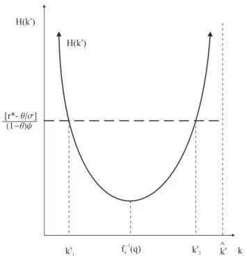
Substituting (1) into (8) and rearranging terms, we find that the government budget is in balance att+ 1if banks follow strategy 1att, and if. Thus, any equilibrium value of ηt for which banks follow strategy 1 (2) must follow the upward sloping portion of lie.
6 Steady state equilibria
There is a stable equilibrium in which banks follow strategy 1 at any date if (19) and (20) are satisfied. Of course, a related proposition applies to the existence of a stable equilibrium in which banks follow strategy 2 for all time.
7 Comparative statics
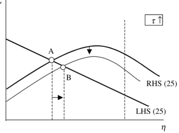
A change in τ
Another possibility is that a steady state equilibrium exists where banks follow strategy 1 before the increase in τ. In this situation, the increase in iτ implies that there is no longer a steady state where banks follow strategy 1.
A change in the deposit insurance premium
Changes in reserve requirements
8 A comment on risk-based deposit insurance premia
9 Conclusions
A preview of the results, as well as a deeper motivation of the model, is presented in Section 2. In Section 4, I present a benchmark version of the model in which the nonbank public uses outside money and there is no intermediation.
2 Preview of results and literature review
After careful research, [8] identifies three key ingredients of the role of banks in the Diamond and Dybvig model. That is why having internal money available to spend increases the attractiveness of the intermediary capital mechanism.
3 The environment
One of the simplifying assumptions in my model is that capital actually remains idle in the hands of a consumer, and so there is apparently no opportunity cost to transfer this capital to a producer. It can be shown that this value, divided by two, corresponds to the expected discounted utility that each nonbanker faces at the very first date of the economy.
4 Benchmark allocations
If there are 1-potential producers with money in the current period, while πpq producers (without money) engage in trade in the current period, then the next-period measure of consumers with money is given by 1−p+πpq. The requirement of stationarity forq is thus. By Lemma 2, economy-wide welfare maximization, min{Ub, Un}, for π < 1, would require a greater allocation of capital to the non-banking sector, that is, kn> kb, so that Ub=Un .
5 Credit allocations
It is shown in the proof that the determinant of the matrix M,det(M), is positive and converges to zero as β approaches one. I present in a lemma below, for the sake of completeness, the full description of the allocation of capital in the banking sector when intermediation takes place.
6 Concluding remarks
There exists an open interval K⊂(0,3) of capital levels such that, if k∈Kandβ is sufficiently high, capital intermediation is essential, in the sense that bankers trade capital with non-bankers with positive probability in an optimal situation. However, the model can provide new insights compared to [5], because the banks here are never illiquid in the sense of fiat assets.
Appendix
Financial fragility in small open economies
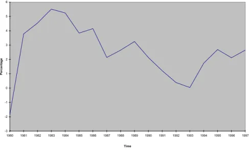
Indeed, each of the episodes of the Mexican crisis coincided with a notable increase in the world interest rate (Figure 2). 4. Alternatively, domestic borrowers can provide the world rate of interest in an economy with a relatively high capital stock in the tradable sector and thus a high level of income.
3 Trade
Factor markets
One unit of tradable good invested at time yields one unit of sectorbcapital at time+ 1.All agents, regardless of their type, have access to the typebcapital investment technology.13.
Credit markets
It is also straightforward to demonstrate that the expected utility of a funded borrower under credit rationing is given by. the expected payoff of a funded entrepreneur can be written asφrat+1−rt[q−wt]. We observe that the parameter φ represents the expected amount of type of capital produced per unit invested, net of monitoring costs, when credit is rationed.
International asset flows and money
From now on, we analyze equilibria in which credit is rationalized and potential entrepreneurs prefer borrowing to lending. Therefore, all potential entrepreneurs would prefer to run their own investment projects, but only some of them will actually receive the external funds necessary to do so.
4 General equilibrium
- The first period
- Steady-state equilibria
- Comparative statics
- Dynamics
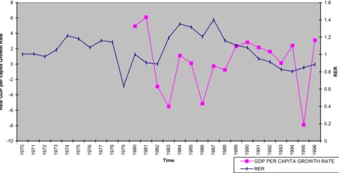
We find that the steady state with high output and low RER is a sink when global interest rates are “low enough”. An unexpected increase in the global real interest rate, causing it to exceed its critical level, would eliminate all equilibrium paths close to the steady state with high output and low RER.
5 Conclusions
Proof of Lemma 2
Proof of Lemma 3
Inflation, growth and exchange rate regimes in small open economies
In this sense, there may be a real cost to implementing a fixed exchange rate regime. Next, in Section 3, I consider a model of a small open economy operating under a fixed exchange rate regime.
2 A flexible exchange rate regime
- The environment
- Trading and financial intermediation
- Agents’ behavior and factor markets
- Loan contracts
- A general equilibrium
- Dynamic equilibria
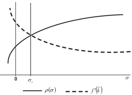
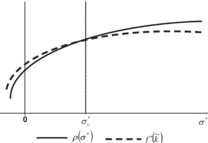
Statement 2. An increase in either the steady rate of inflation in the rest of the world (V*) or the international interest rate on deposits (r) reduces the capital-labour ratio (kˆ) and increases the ratio of investment abroad to total saving (Fˆ) in a Walrasian steady-state equilibrium. Then an increase in the domestic inflation rate increases (decreases) the steady capital-labour ratio k~.
3 A fixed exchange rate regime
Government policy
For high values of V, 1-T+D>0 and 1+T+D<0, the equilibrium state becomes a saddle with a positive stable eigenvalue;. T gives foreign "currency" reserves held against the domestic money supply measured in foreign currency units.
Stationary equilibria
In a pure fixed exchange rate regime, an increase in r has no direct effect on government finances, and G remains unchanged. These properties are independent of how the domestic money supply is supported in a fixed exchange rate regime.
Dynamic equilibria
For high levels of foreign inflation the steady state is still a sink, dynamic equilibria are indeterminate but dynamic paths will exhibit damped oscillations. In a purely fixed exchange rate regime, the steady state is always a sink with real and positive eigenvalues.
4 Conclusions
Financial arrangements and dynamic inefficiencies
Contingent damage prices are constructed under two assumptions regarding net and equilibrium consumption allocations are derived. While contingent damages prices are fixed, other prices, such as nominal prices, can vary.
2 Description of the economy
Central planning problem
Peled ignores the utility of the initial old generation and thus focuses on the steady state. The Pareto optimal solution of equal treatment (ET-PO) shows a constant marginal degree of substitution between states or
3 Competitive equilibrium
Deterministic and autarkic solutions
3 If an economy is dynamically inefficient, then the discounted present value of the fund flow is infinite. Therefore, the Lagrange multiplier μt(st) can only be expressed as a function μ(st) of the current state.
Equal treatment futures market
A young agent chooses current consumption and state-contingent elderly consumption such that the weighted marginal utilities are equal. To find the stationary solution in which a young agent takes out full insurance against capital risk, both young and old, consider that the budget constraint can be expressed as: 40) so that µt=µt(st) is constant across statest.
4 Equivalent financial mechanisms
- Optimal transfers
- Financial mechanisms
- Social security
- Financial intermediary deposits
Therefore, the conditional distribution of the futures market can be achieved by issuing a constant money supply in the initial period of the model. In the case of the ET-PO equilibrium, the distribution can be supported by a special money growth rule.
5 Conclusion
Deposit insurance is "mispriced" in that the expected discounted present value of the return on the purchase of the insurance is not necessarily equal to the price(s) per unit of insurance. 5.] Manuelli, R.: Existence and optimality of currency equilibrium in stochastic nested generation models: the pure endowment case.
I examine the implications of different transfer schemes under two concepts of Pareto optimality for the market price of risk. The market prices of risk for competitive ET-PO and CPO equilibria are compared in Section 3.
1 Description of the economy
Contingent claims matrix
The elements of the matrix Q are the quota demand prices that support consumption allocation(s), w(s)−c(s). In the OG model examined here, SDF is the product of MRS times the ratio of marginal utilities of tomorrow's youth relative to today's youth.
Pareto optimal allocation
As mentioned earlier, Aiyagari and Peled show that a necessary and sufficient condition for a Pareto optimal allocation to exist is that the matrix has a dominant root that is less than or equal to unity. A conclusion drawn here is that the associated within-period MRS matrix, the K matrix, must have a dominant root less than or equal to unity for a Pareto optimal allocation to exist.
2 Optimal transfers
Autarky
Therefore, the existence of a Pareto optimal solution will depend on the dominant root of the matrix P, which depends on the transition matrix Π, and the properties of the diagonal matrix K. Therefore, if the sequence of conditional damage prices fails to converge in (5), this will be the result of the size of the dominant root in the matrix K , IAS within the period.
Equal treatment pareto optimal allocation
Under Assumption 1, specifically that the endowment allocation is bounded such that young agents want to save, the allocation of the endowment across agents within a period will not affect the contingent demand matrix Q. While the size of the transfers will be determined by the endowment distribution, ET-PO matrixQ not be affected.
3 Asset pricing implications
Then any first-period allocation within this interval will not change the consumption allocations and therefore will not affect matrixQ. The optimal transferxf can be made by the sale of contingent claims and by state-contingent taxation, as discussed in Labadie [2004].
4 Conclusion
The distribution of the distribution within a period is an important determinant of the price matrix Q. The order of powers of the price matrix determines the time series properties of the SDF and subsequently for asset prices and returns. A lower bound on the market price of risk and on the variance of the SDF is also established and the dependence of these bounds on the variance of the within-period MRS and the intergenerational IMRS is also demonstrated.
Money
The distribution of money and its welfare implications
The use of lotteries on transfers of indivisible money balances can capture some aspects of the idea of divisibility of money, while maintaining manageability. Indeed, recent work suggests similarities between divisible money models or indivisible money lotteries.1 This note explains what aspects of money divisibility lotteries can and cannot capture.
2 Environment
The problem with this is that buyers spend none or all of their money, but never portions of it. The reason is the large distributional effects present when agents can spend portions of their balances.
3 Symmetric stationary monetary equilibria
Indivisible balances and lotteries
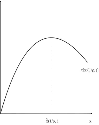
A high curvature of the utility function, large γ, and low trade frictions, small ρ, give buyers an incentive to spread consumption over time. As the curvature of the utility function or trade frictions decrease, there is an incentive to spend even less, and the equilibrium probability decreases.3.
Partially divisible balances without lotteries
7Since {Vb+d−Vb} is a decreasing sequence, ρsmall and γlarge satisfy(qs)> V1/N. fors= 0. The poorest buyer spends everything he has even if the price is high. The richest buyer spends the least he can, even if the price is low. ρfalls) future consumption is discounted less, so buyers are less likely to delay a trade to search for a better price.
Divisibility and distributional effects
This makes sense, since in an economy where N = 1, the value of money (hence q) also falls by M >0.5. The redistribution of money it creates relative to the economy (ii) is so beneficial that it overtakes the inefficiency of trading due to the rigidity of money supplies (spendd= 0.5ord= 1).10.
4 Final remarks
It follows that the probability of a money transfer increases in the buyer's wealth, but decreases in the seller's. In this case, {m0(t), .., mN(t)} defines the distribution of money in the economy, a probability measure of N that must satisfy M =N.
3 Symmetric stationary monetary equilibrium
Terms of trade
We use the generalized Nash protocol whereθ∈[0,1] is the buyer's bargaining power, and1−θ is the seller's. The seller produces goods qs,b(d) for the buyer and, conditional on qs,b(d), the buyer gives money to the seller with probability τs,b(d) and nothing else.
Value function
A second interesting result is that, given quantities and value functions, the probability of the money transfer decreases in the buyer's bargaining power, τs,bis decreasing in θ. The parameter γ, the inverse of the intertemporal elasticity of substitution, appears due to the specific CRRA formulation of preferences.
4 Characterization of equilibrium in a special case
Stationary distributions
The second term implies that sellers with n − 1 units of money can get another unit with probability N. This similarity occurs despite (i) very different underlying equilibrium consumption patterns and (ii) even when N is relatively small (see Figure 1 ), which significantly limits an individual's ability to spend small portions of the money balance.
Individually optimal strategies
This reduces the seller's willingness to produce per unit money, which is bad for the buyer. Consider a match(b, s) = (N,0) where the buyer's incentive to spend more than one unit of money is the strongest.
Numerical experiments show that as money becomes more divisible, these inefficiencies decrease as the distribution of money becomes more concentrated around the mean. Such questions include the effects of money creation on welfare and on the distribution of prices and money.
6 Appendix
Price dispersion, inflation and the value of money
Money, price dispersion and welfare
Environment
For any other good, the household's preference decreases with the distance (ie, the shortest arc length) between the good and the preferred good. In addition, household members are assumed to act in the best interests of the household.
A particular household’s decisions
Matching is characterized by the distance of the producer's goods from the buyer's preferred goods, z, and the buyer's monetary holdings, m/N. In this case, the buyer spends all of his money, and the quantity of goods traded is less than the quantity that maximizes the total trade surplus.