Business Statistics for Competitive Advantage

Building Multiple Regression Models

Model Building and Forecasting with Multicollinear Time Series

Indicator Variables

Nonlinear Multiple Regression Models

Logit Regression for Bounded Responses

Index 405

Preface

Later chapters include sample memos for students to use as templates, making communicating statistics for decision making an easy skill to master. Preliminary editions of Business Statistics for Competitive Advantage were used at the McIntire School, University of Virginia, and I thank the many bright, motivated, and enthusiastic students who provided comments and suggestions.

Statistics for Decision Making and Competitive Advantage

Statistical Competences Translate Into Competitive Advantages
Attain Statistical Competences And Competitive Advantage With This Text
Follow The Path Toward Statistical Competence and Competitive Advantage
Use Excel for Competitive Advantage
Statistical Competence Is Satisfying

It is useful to begin model building with the simplifying assumption of constant response, but it is essential to. The approach to modeling is steeped in logic and begins with logic and Modeling with simple regression begins in Chapter Four and occupies the focus.

Describing Your Data

Describe Data With Summary Statistics And Histograms

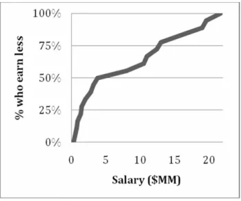
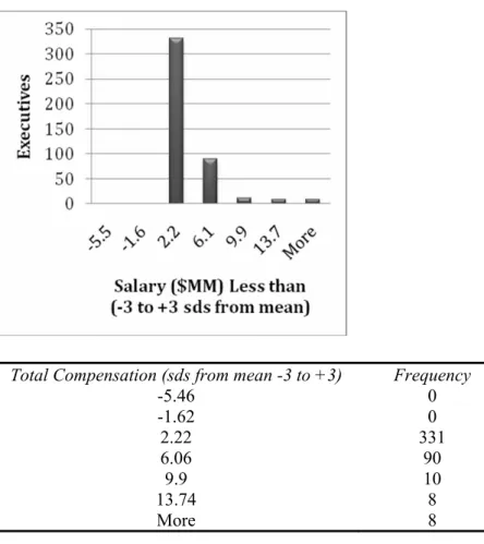
In addition, he needs to know how unusual extreme salaries are in order to better evaluate the offer. I would like to know if the rookie will be in the higher paying half or not.

Table 2.2 Yankees sorted by salary (in $MM)

Outliers Can Distort The Picture

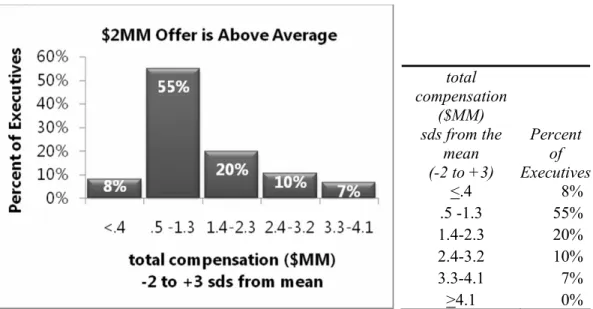
Each collects a compensation package of more than $13.7 million, a compensation level that is more than three standard deviations greater than the mean. More than three-quarters of directors earn less. Because exceptional directors exist, the original distribution of compensation is skewed in that relatively few exceptional directors are unusually well compensated.

Figure 2.3 Histogram of executive compensation

Round Descriptive Statistics

Central Tendency and Dispersion Describe Data

Data Is Measured With Quantitative or Categorical Scales

We can sort the nominal data to find the best known number that occurs most often, the mode, which we use to report central tendency. As with other categorical data, we rely on reporting the central tendency of ordinal data.

Continuous Data Tend To Be Normal

Between quantitative and categorical scales are ordinal scales that we use to rank order data, or to convey direction but not magnitude. With ordinal numbers, we can order the data, but we cannot add, subtract, divide, or multiply the order.

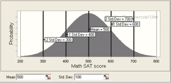
The Empirical Rule Simplifies Description

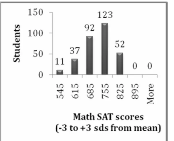
Class of '06 math SAT scores are approximately Normally distributed with a mean of 685 and a standard deviation of 70. Relative to the larger population of all SAT takers, the smallest standard deviation in the class of students' math SAT scores '06, 70 vs. 100 , indicates that Class '06.

Figure 2.8 Histograms and descriptive statistics of class ‘06 math SATs

Describe Categorical Variables Graphically: Column and PivotCharts

Descriptive Statistics Depend On The Data

Produce descriptive statistics and view distributions with histograms Executive Compensation. We will describe executive compensation packages by

In the Executive Compensation file, select C1, [Enter], to paste the histogram bins formulas into columns C through E. In C2, replace the zero mean with the sample mean by entering =B450 [Enter]. For Bin Range, select E1 and then use shortcuts to select the histogram bins in column E with Ctrl+Shift+Down arrow.

Sort to produce descriptives without outliers

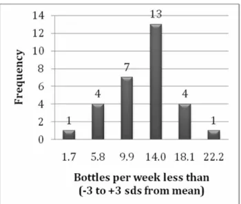
Histogram bin formulas will automatically update the bin thresholds with your new mean and standard deviation.). Update the descriptive statistics in B450:B454 and rerun the histogram with only rows with compensation less than $7.9 million, B1:B429.

Plot a cumulative distribution

To determine Normality, we want to see the sample percentages that are -3 to +3 standard deviations from the sample mean. Copy and paste the histogram bins.xls formulas into the Excel 2.4 SATs ’06.xls file in columns E, F, and G, then change the mean and standard deviation to those of the sample:.

Produce a column chart from a PivotChart of a nominal variable

H IC to select the Home menu and Insert function and to insert a column to the left of the selected cell or column. N/A to select the Insert function, the Pivot menu, and to insert a PivotTable NX to select the Insert function and insert a text box.

Descriptive Statistics

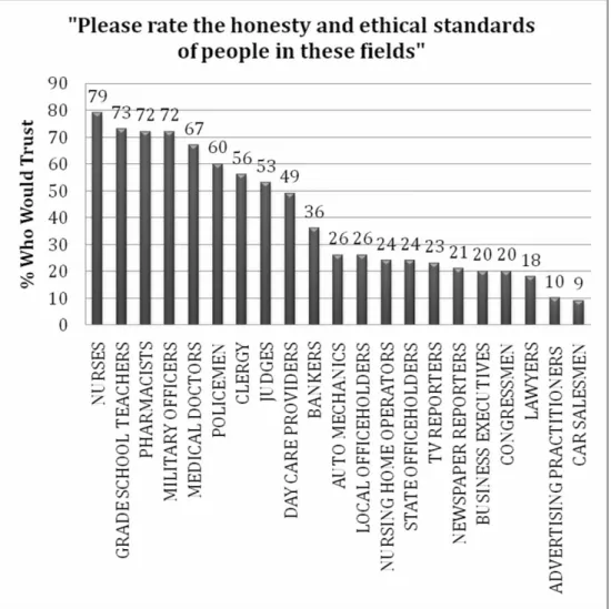
Create a Pivot Table and Pivot Chart (column chart) comparing the percentages of Add a label summarizing the survey results. See your text for a similar example in Excel.). Managers of a political campaign are considering launching an effort to enlist the support of Hollywood celebrities.

Procter & Gamble’s Global Advertising

VW Backgrounds

Hypothesis Tests, Confidence Intervals and Simulation to Infer Population Characteristics and Differences

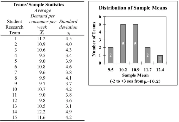
Sample Means Are Random Variables
Use Sample Data to Determine Whether Or Not μ Is Likely To Exceed A Target
Confidence Intervals Estimate the Population Mean From A Sample
Round t to Calculate Approximate 95% Confidence Intervals With Mental Math
Margin of Error Is Inversely Proportional To Sample Size
Samples Are Efficient
Use Monte Carlo Simulation with Sample Statistics To Incorporate Uncertainty and Quantify Implications Of Assumptions
Determine Whether There Is a Difference Between Two Segments With Student t

Each of the sample standard deviations is close to the true, unknown population standard deviation σ=4. Rule of thumb, we know that sample means are within about two standard errors of the population mean 95% of the time.

Segment Income

Confidence Intervals Complement Hypothesis Tests

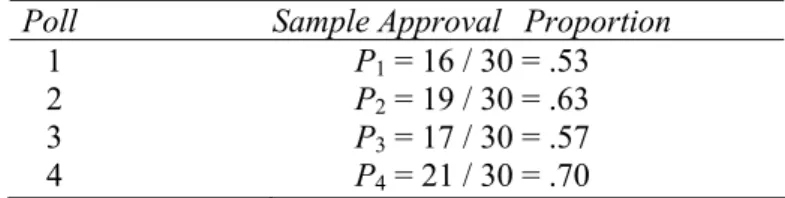
Concerned managers have hired four public opinion polling organizations to find out whether medical testing on animals is acceptable or not. With much larger samples and correspondingly smaller margins of error, it becomes clear that the majority approves of medical testing on animals.

Table 3.6 Sample approval proportions by poll

Conditions for Assuming Approximate Normality to Make Confidence Intervals for Proportions

Conservative Confidence Intervals for a Proportion

Sixty-one percent of American adults agree that medical testing on animals is morally acceptable.

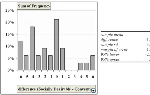
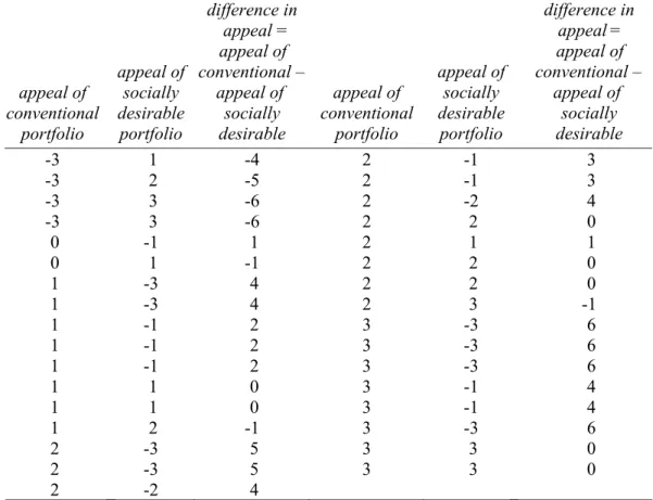
Assess the Difference between Alternate Scenarios or Pairs With Student t

Based on sample evidence, shown in Figure 3.10, we conclude that a "socially desirable" label reduces portfolio attractiveness. Investors rate the attractiveness of "socially desirable" portfolios by approximately 1 to 3 points on a 7-point scale, relative to other equivalent portfolios.

Table 3.10 Paired ratings of other & socially desirable portfolios

Inference from Sample to Population

Test the level of a population mean with a one sample t test

Make a confidence interval for a population mean

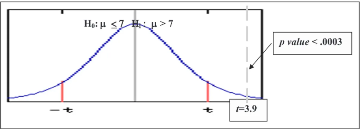
Find the p-value for this t using the Excel function TDIST(t,df,tails), entering t in B36.

Illustrate population confidence intervals with a clustered column chart

To see the confidence intervals for the abandoned call rating and the static rating, select C34:C38 and then use keyboard shortcuts to fill in statistics for the abandoned call rating and the static rating. To see the confidence intervals for all three service dimension ratings, first insert a row above row 37 for chart labels, using.

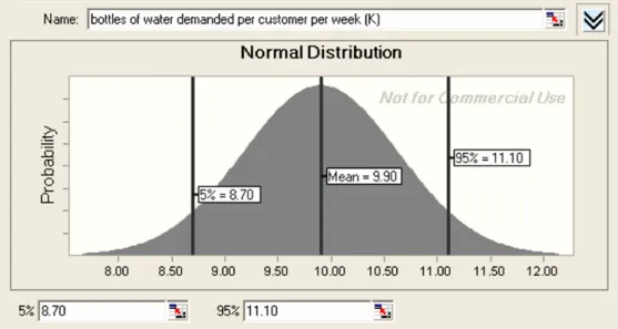
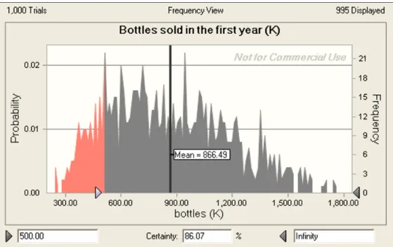
Conduct a Monte Carlo simulation with Crystal Ball

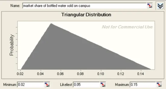
You will see the simulated distribution of bottles sold in the first year, given the assumptions. Based on the assumptions, there is an 86% chance that demand will exceed 500 (K) bottles in the first year.

Test the difference between two segments with a two sample t test

Procter & Gamble management wants to know if household income is a good basis for segmenting the market for their new preemie diapers. We will test the hypothesis that average income is greater in the segment that is likely to try the new diapers than in the segment that is not likely to try.

Construct a confidence interval for the difference between two segments

Illustrate the difference between two segment means with a column chart

Construct a pie chart of shares

Test the difference in levels between alternate scenarios or pairs with a paired t test

AY2 to select the Data and Analysis Data menus AS to select the Data and Sort menus. Select all filled cells in a column: select the first cell in the column, then Cntl+Shift+Down Arrow.

Inference

Dell PDA Plans

Bottled Water Possibilities

Immigration in the U.S

McLattes

A Barbie Duff in Stuff

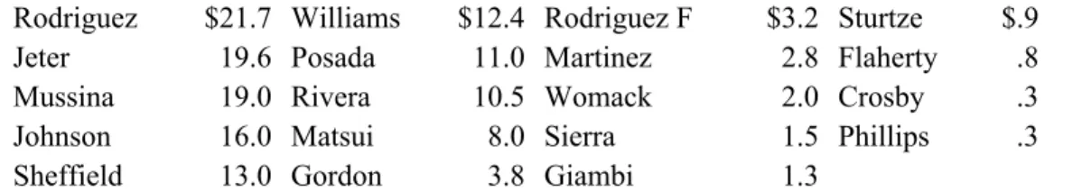
Yankees v Marlins: The Value of a Yankee Uniform 1

Gender Pay

H0: The taste rating of Seagram's Polish Vodka is at least as high as the taste rating of Stolichnaya. H1: The taste score of Seagram's Polish Vodka is lower than the taste score of Stolichnaya.

Pulaski Taste.xls are repeated measures. From These experimental data in

The average difference between the taste ratings of Polaski vodka poured from a Stolichnaya bottle and Polaski vodka poured from the Seagrams bottle with the Polaski brand name is not greater than zero. H1: The average difference between the taste ratings of Polaski vodka poured from the Stolichnaya bottle and Polaski vodka poured from the Seagrams bottle with the Polaski brand name is positive.

American Girl in Starbucks

Mattel executives believe that about 25% of those who know the film will purchase tickets, although this percentage could be as low as 10% or possibly as high as 60%. Mattel and Warner Brothers also consider McDonalds as a potential promoter of the new film.

Quantifying the Influence of Performance Drivers and Forecasting: Regression

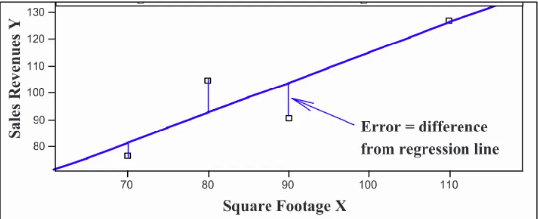
The Simple Linear Regression Equation Describes the Line Relating A Decision Variable to Performance

Footage Line Fit Plot

F Tests the Significance of the Hypothesized Linear Relationship, Rsquare Summarizes Its Strength and Standard Error Reflects

The difference, SST - SSE, also called the regression sum of squares, SSR or model sum of squares, is the portion of the total variation in Y that is affected by variation in X. This ratio is distributed as an F with 1 numerator (for the predictor ) and (N-2) denominator degrees of freedom:. We lose one degree of freedom when estimating the mean of the dependent variable and one when estimating the mean of the independent variable.) The percentage of total variation in the.

Figure 4.2 Four errors from the regression line

The Population Slope Is Tested And Inferred From Our Sample

From experience and logic, the owner of the kiosk chain had a good idea that snapshots have a positive effect on revenue, so his alternative hypothesis is that the slope is positive. There is less than a twenty percent chance that sample data would be observed if the recordings did not generate revenue.

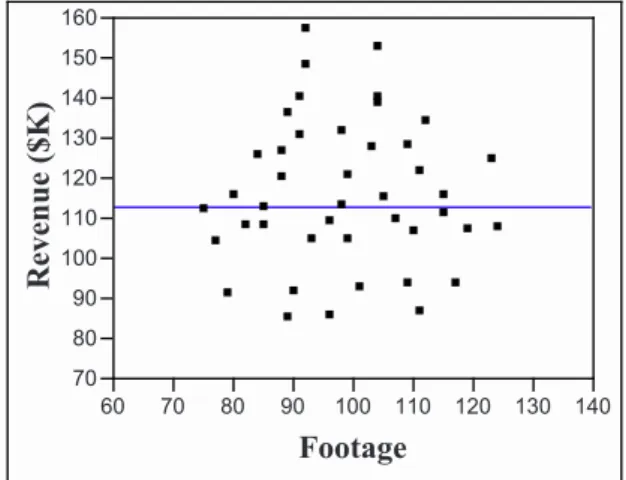
Figure 4.3 X does not drive Y and the regression line slope is flat (b 1 =0)

Analyze Residuals To Learn Whether Assumptions Have Been Met

Histogram

Predicted and Actual Revenue ($K) by Footage

Use Sensitivity Analysis to Explore Alternative Scenarios

If, for example, the kiosk chain owner expected to add thirty new kiosks of the same size and wanted to know what average earnings he could expect, he would ask for the 95% conditional mean prediction interval, given the planned kiosk size. 95% Mean Prediction Intervals for Mean Earnings of Varying Sizes If we are interested in estimating the mean population performance given a particular.

95% Conditional Mean Prediction Intervals and Actual Revenues by Footage

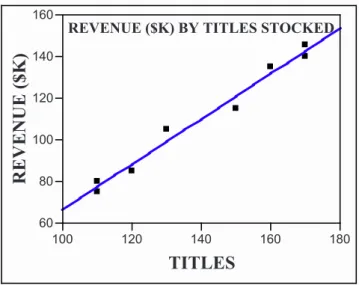
Explanation And Prediction Create A Complete Picture

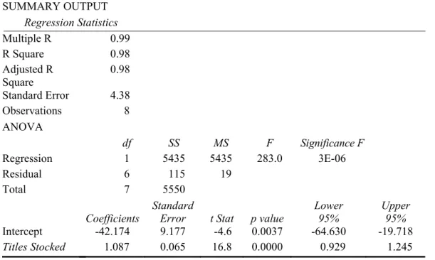
Variation in admissions accounts for 86% of the variation in turnover among a random sample of 52 stores. The HitFlix owner presented the results of his regression analysis by illustrating the regression line with 95% confidence prediction intervals on top of the actual data.

Present Regression Results In Concise Format

For the general business audience, the verbal description with graphic illustration conveys all the important information. The additional four lines provide the information that statistically literate readers will want to assess how well the model fits and which parameter estimates are significant.

We Make Assumptions When We Use Linear Regression

Correlation Is A Standardized Covariance

In this case, all the points on the scatterplot would fall on top of the regression line. Note that although X and Y in the third panel are not linearly related, they are strongly related.

Figure 4.8 Movie rental kiosk revenues ($K) by titles stocked

Correlation Coefficients Are Key Components Of Regression Slopes

In the concept test of the new preemie diaper with a sample of 97 preemie mothers, price sensitivity was measured as the difference between trial intentions at competitive prices and premium prices, each measured on a 5-point scale (1 = "Definitely Will Not Try" . to 5 = "Definitely going to try"). While it doesn't have a big impact on price sensitivity, fit does matter, along with other factors.

Table 4.8 Regression of revenue by titles

Correlation Summarizes Linear Association

Linear Regression Is Doubly Useful

For Input Y Range, Observations on Dependent Variable, Income ($K), select B1, then use shortcuts to select cells in B: Cntl+Shift+Down Arrow to B53. For Input X Range, observations in the independent variable, views, select A1, then use shortcuts to select cells in A: Cntl+Shift+down arrow to A53.

Fit a simple linear regression model

We will use regression analysis to explore the linear impact of views differentials on revenue differentials ($K) in a random sample of 52 movie rental kiosks. In the population of HitFlix movie rental kiosks, the expected difference in revenue due to a unit change of one square meter of Movie is in the range of .99 to 1.25.

Construct prediction and conditional mean prediction intervals

In F2, enter the formula for the lower bound of the 95% prediction, the prediction minus the margin of error of the prediction. In G2, write the formula for the upper bound of the 95% prediction, adding the prediction plus the margin of error of the prediction.

Find correlations between variable pairs

WFR to select the View and Freeze Panes menus, and for Freeze Rows JAB to select the Layout and Data Labels menus. JARM to select the layout, error bar and custom error bar menus JAT to select the Layout and Title menus.

Regression

How much variation in the importance of thinness is explained by variation in each of the demographics. Find the 95% confidence interval for the difference in slenderness significance associated with a unit difference in each demographic in the population.

GenderPay.xls contains employee salaries and levels of responsibility from a random sample of employees

Slam's Club's head of human resources was shocked by recent revelations of gender discrimination by Wal-Mart ("How Corporate America is Betraying Women," Fortune, January, but believes his company's wages reflect a level of responsibility (and no He asked you to analyze this hypothetical relationship between level of responsibility and salary.

GenderPay (B)

Your client is a busy executive and in the near future will only have enough time to read a single page of analysis, single spaced, in 12 pt font.

GM Revenue Forecast 1

What percent of the variation in income can be accounted for from the past How close to current income can you expect a forecast to be 95% of d.

Impact of Defense Spending on Economic Growth

Marketing Segmentation with Descriptive Statistics, Inference, Hypothesis Tests and Regression

Segmentation of the Market for Preemie Diapers

P&G Targets the ‘Very Pre-Term’ Market Wall Street Journal

Demographic Information
Attribute Importance
Revenue Potential
Additional Information Needed

Write Memos that Encourage Your Audience to Read and Use Results

Derive the expected market share ratio of the population from the sample ratio that would try Pampers Preemies at the value price (Value Trier=1). Bottom line first, above, in the title.” Your audience has seconds to digest your slide.

MEMO

Fit Importance Drives Intent

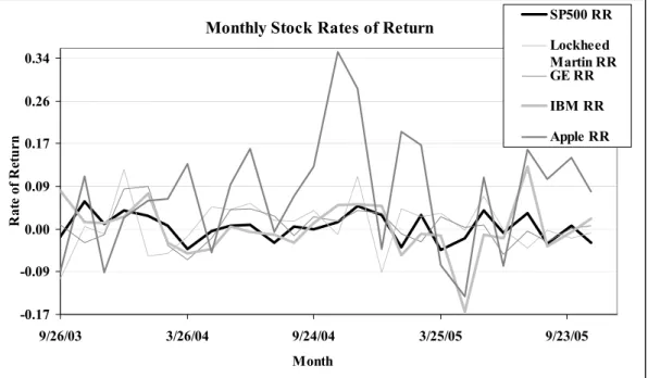
Rates of Return Reflect Expected Growth of Stock Prices

Goldman Sachs & Risk-Free prices

Yahoo & Risk-Free Prices

Investors Trade Off Risk And Return

Compared to a market index, such as the S&P 500, a composite of 500 individual stocks, many individual stocks offer higher expected returns, but at greater risk. Like other weighted averages, a market index has an expected rate of return at the midpoint of the expected returns of the individual stocks that make up the index.

Beta Measures Risk

A one percent increase in market value is associated with an expected change in share price of more than one percent. A one percent change in market value is associated with an expected change in share price of less than one percent.

Figure 6.3 Monthly rates of return of four diverse stocks and S&P500 November 2000 – October 2005

A Portfolio’s Expected Return, Risk and Beta Are Weighted Averages of Individual Stocks

Efficient Frontier

Efficient Frontier: Expected Rate of Return by Risk

Estimate portfolio expected rate of return and risk
Plot return by risk to identify dominant portfolios and the Efficient Frontier
Individual Stocks’ Beta Estimates
Expected Returns and Beta Estimates of Alternate Portfolios
Portfolio Comparison
Portfolio4.xls contains five years of monthly data on

Portfolio risk depends on the covariances between individual stocks' rates of return and the market rate of return. Monthly rates of return for the other three-share portfolios were similarly calculated in C to E.

Association between Two Categorical Variables: Contingency Analysis with Chi Square

Chi Square Tests Association between Two Categorical Variables
Chi Square Is Unreliable If Cell Counts Are Sparse
Simpson’s Paradox Can Mislead
Contingency Analysis Is Demanding
Contingency Analysis Is Quick, Easy, and Readily Understood
Use chi square to test association

Since the components of chi square include the expected number of cells in the denominator, rare (with an expected number less than five) cells increase the chi square. We are interested in the percentage of each age group that chooses Made In U.S. cars.