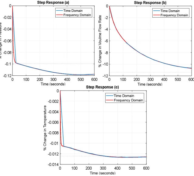
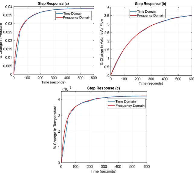
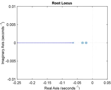
Responses of original and reduced order models for g s31( ) Figure 5.1 d Responses of original and reduced order models for g s12( ) Figure 5.1 e Responses of original and reduced order models for g22( )s Figure 5.1 f Responses of original and reduced order models for g32( )s Figure 5.1 g Responses of original and reduced order models for g s31( ) Figure 5.1 h Responses of original and reduced order models for g32( )s Figure 5.1 i Responses of original and reduced order models for g s33 ( ) Figure 5.2 Root locus graph showing that two poles overlap with the.
Research Background
- HVAC Systems Overview
- HVAC System Major Components
- HVAC Systems Performance Challenges
- Physical fundamentals Governing HVAC System Operations
In a single-channel system, either the cooling or heating function can be used, but not both. The thermal conductivity of a material is an indicator of the ease of heat transfer in the material.
Research Problem
Therefore, the reliability of the control system is a major requirement when operating the HVAC system under input changes, disturbance effects, and fault conditions with the aim of ensuring cost-effective, safe, and efficient system operations. The HVAC system has distributed components such as vented volume where lumped modeling is not the right option.
Research Significance
The control system should also enable disturbance suppression and restoration of the system operations to normal performance in a relatively short time. Another important significance of the study can be realized from the least control efforts spent on achieving the control targets and especially while rejecting the disturbance applied to the system outputs.
Research Aims and Objectives
Research Aims
The Performance Index (PI) equation, which is part of the general control energy expression and can be calculated by finding the integral of the summation of the squared control signals, is used to optimize the control energy consumption. The control technique used in this study is Least Effort Control where it uses specific values of forward gains and feedbacks corresponding to the minimum values of the Performance Index Equation.
Research Objectives
Research Organization
Hence, identifying a reliable multivariable mathematical HVAC system model that is close to reality is one of the main research goals. An overview of the HVAC system types, structures, design gaps and challenges is part of the chapter.
Physics-Based Modelling
The output of the model, represented by the internal temperature, was influenced by external heat sources (i.e. the heat flux generated by the external air temperature and solar radiation on the walls). However, the flat capacitance model of the radiator did not consider the time delay of heat transfer.
Data-Driven Modelling
Based on the data obtained, the input-output relationship of the system model can be derived by using certain mathematical techniques (for example, statistical regression by mathematical processing). A data mining algorithm is part of the data-driven modeling or black box technique; it is a technique defined by Hughes (2017) as.
Grey Box Modelling
To identify the values of the model parameters, which are basically five parameters related to the thermals. It is worth noting that the identified system parameters in the gray box models must be reviewed and verified in case the operating conditions deviate, with the aim of maintaining the accuracy of the model.
HVAC Distributed Parameter Modelling
The model itself has no dimensional information, and all the effects of the multiple thermal capacitance, inductance, and resistance elements exist at undefined points in space. Also, the model generates dimensionally large matrix models and the accuracy of the model depends on how many lumped elements to use without guidance for the number of elements to incorporate.
Summary of HVAC System Modelling Techniques
A data-driven or black-box modeling methodology, which could be an alternative to physics-based models, is a simple modeling solution, but has a major disadvantage in that when the original system conditions or training data of the HVAC system that were then discussed, the derivation of the model change, the accuracy of the model will deteriorate significantly. Neglecting such system specificity will not help to realize a reliable or robust HVAC system model, and therefore you may encounter fragile system design and poor performance.
Mathematical Model to be Employed in the Study
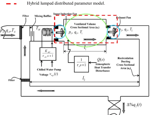
As mentioned in the previous section, due to the accuracy and closeness to reality of the HVAC system between different models assessed, the Hybrid Distributed Lumped Parameter Model is the recognized mathematical model to be used in this study. The temperature variations occur when the HVAC system is operating and cause changes in airflow pressure and airflow velocity and can be caused by external environmental changes so such temperature variations lead to transient heat transfer effects.
Chapter Summary
Therefore, the control of industrial processes with time delay can be a challenging task as such time delay creates phase shifts, where the phase shift in feedback control usually causes limitations on the control bandwidth which in turn affects the stability of the closed loop system. The dynamics and the set points of the system are time variant and affected by many disturbances.
Classic Control Techniques
With SISO systems, a test phase can be implemented so that the input and output data of the process is collected. After completion of the testing phase, data can be analyzed to realize the process model for a range of operational values to identify appropriate PID controller parameters.
Advanced Control Techniques
Robust Control is one of the control techniques that has also been used to control HVAC systems. The Robust Control technique is used to ensure the performance of the system under control regardless of the changes in the system dynamics.
Multivariable System Control
The authors used real experiments combined with simulations to prove the effectiveness of the proposed control technique. The inclusion of the concept of optimization in the feedback of the proposed control technique is called Optimal Control.
Least Effort Multivariable Control Technique
The control strategy based on the minimization of control energy has emerged from the British School of Control and is called the least effort (LE) control technique. The solution proposed here also aims to obtain improved system dynamics, accurate steady-state responses, minimal coupling of internal loops, and minimal power control dissipation to recover from disturbances affecting the system.
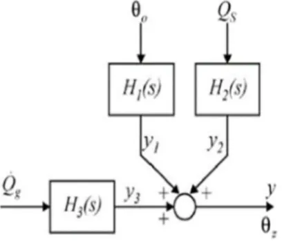
HVAC Hybrid Distributed-Lumped Parameter model
Airflow temperature changes caused by changes in air pressure and air flow at the inlet of the ventilated volume. Airflow temperature changes caused by changes in air pressure and airflow at the outlet of the ventilated volume.
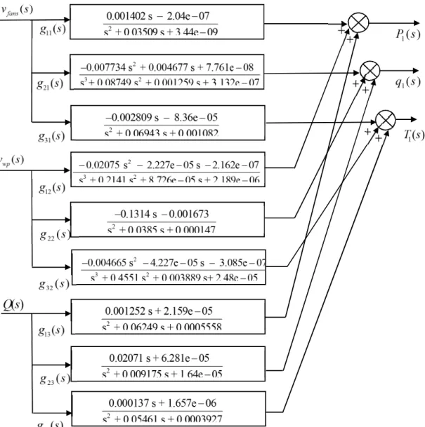
Deriving the Air Conditioning System Transfer Function Matrix
Fast Forier Transform (FFT)
It processes the time domain signal by observing and measuring when the signal passes through cycles so that amplitude, rotational speed and offset of each different cycle are defined and calculated. Therefore, using FFT is not the most efficient technique to obtain the system representation in the frequency domain for this study.
System Identification Toolbox
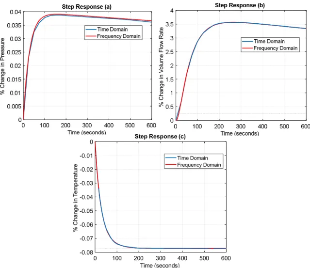
MATLAB in this study will aim to use the time domain data as illustrated in Figures 4.3, 4.4 and 4.5 to extract the continuous time transfer function in Laplace transform representation. Similar tables of the remaining time domain responses have been identified and fed to the SIT application.
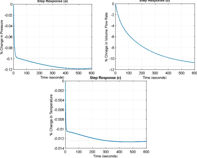
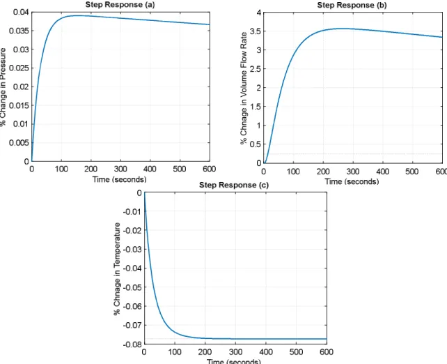
Air Conditioning Multivariable Open Loop Responses
Input of 1% step change in vt1( ) and v t2( ) simultaneously with 0% change in all other inputs causes the air pressure at the inlet of the ventilated volume to increase exponentially from. When an input change of 1% occurs in the atmospheric ambient heat transfer change with 0% and in the ventilated volume ( )Q t at all other inputs, a corresponding increase in temperature will be encountered at the input volume of ventilated.
Control Objectives
Consequently, reducing the coupling between the outputs should be one of the control objectives, so that when any of the inputs is changed, the effect on the other system outputs will be as small as possible. An acceptably low switching percentage between outputs is also one of the control objectives and must be investigated and confirmed.
LE Control Theory
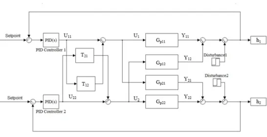
- Closed Loop Plan
- Inner Loop Analysis
- Optimization of the Gains
- Disturbance Rejection Calibrator for LE control technique
- Stability of the System with LE Control
After reference input changes, steady-state, non-interacting responses can be obtained according to equation (4.11). From the solution of equation (4.31), the vector of values ( )h can be calculated based on the arbitrary value for ( )k1.
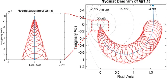
Direct Nyquist Array (DNA)
System Decoupling
Similarly, a column in a matrix is graphically dominant when the union of circles is centered with. 4.43) in a certain extended range of frequencies will also exclude the origin of the complex plane. After the system is decoupled with little residual interaction, multi-loop diagonal controllers can be designed to form Gershgorin bands, which aims to graphically examine the stability of any control loop system.
Direct Nyquist Array Stability Theorem
MATLAB and SIMULATION software is the main research methodology and tool used in the research. The application of control techniques will essentially use MATLAB and SIMULATION software due to its high capacity in dealing with big data, where big data is very important in solving complex design challenges (Matlabtips.com.
LE Controller
Inner Loop Configuration
The matrix L s is then resolved in such a way that when ( )A s is multiplied by ( )L s, the product of the multiplication will be the original ( )G s according to equation (5.4). The Root Locus design technique will be used to select a zero and a gain that can improve the transient responses of the system, which can be predicted faster than the open-loop responses.
Root Locus Design
The gain in the root locus plot is chosen to be b00.23 to achieve an improved performance response of the system so that the responses will be faster as shown later. The location of this pole will improve the dynamics of system responses, as shown later, even at a higher speed.
Performance Index
Equation (8.2) in the appendix represents J /n1 which is the partial differential equation of the Performance Index in equation (8.1) with respect to (n1). On the other hand, the partial derivative J /n2 with respect to (n2) is given by equation (8.3) in the appendix.
Multivariable Performance Index Equation Solution
The script file (8.4) as shown in the appendix is developed and executed to find the list of roots that satisfy equation (8.2) and equation (8.3) simultaneously. Once the matrix (P) is calculated and the feedback gain matrix (F) is chosen, the feedback compensators H s( ) in equation (4.13) can be determined automatically. Ss) in equation (4.6) is the matrix that can be determined based on the zero steady-state error requirement.
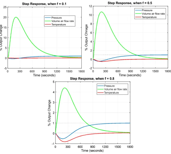
System Performance Analysis under the LE Controller
Such a situation will add some delay to the system responses, which can be clearly seen in the responses of volume air flow ( )P and air temperature ( )T in Figure (5.6). The overshoot of the volumetric air flow response decreases and disappears completely as the value increases (f.
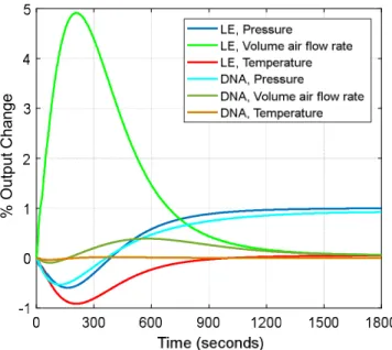
Disturbance Rejection Analysis Under LE Controller
The performance is quite perfect, when the signal 2( )t is applied to the inlet pressure of the ventilated volume. In Figure 5.11, the controller has also managed to recover the influence of the applied disturbance signal 3( )t on the inlet temperature of the ventilated volume.
Direct Nyquist Array
- Decoupling compensators
- Gershgorin Circles
- System Stability Test
- System Performance Analysis under DNA Controller
- Disturbance Rejection Analysis for DNA control technique
The system outputs are decoupled and the cross-talk between the loops is almost zero. In the last part, the performance of the system was investigated under the DNA control system.
Mathematical and Algebraic Operations
A trial and error approach is a known way of finding such a decoupling compensator matrix with no guarantee of the time it will take. However, the mathematical DNA operations were complicated with one major drawback compared to the LE controller, which was an unsystematic trial-and-error approach that created a great challenge to find the decoupling compensator matrix with no specific time to find the solution.
The Controller Simplicity
Unfortunately, there is no clear systematic approach to find an appropriate compensator matrix that separates the plant transfer function. The LE controller avoids the use of integrators and, with simple passive feedback and advanced gains, is much simpler than the DNA technique, which uses very high order compensators (ie 9th to 11th order)).
Closed Loop Responses and Disturbance Rejection
System responses following a unit step change in volumetric airflow output while there are no disturbance changes at. System responses after a unit step change in volume airflow output, while at and there is no disturbance change.
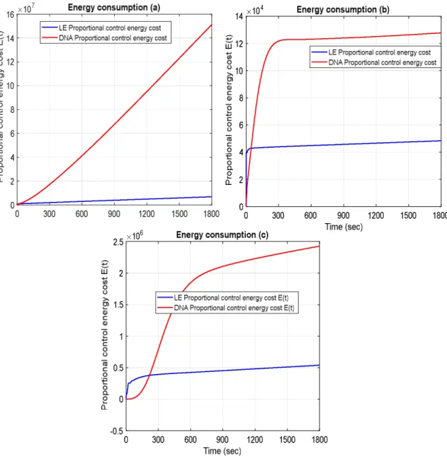
Control Energy Consumption
Proportional control energy costs for disturbance recovery at the system outputs and for operation of the HVAC device are clearly lower in the LE than in the DNA controller for the three conditions. Looking at Figure 6.7, the ratio of the proportional cost of control energy in the LE to the DNA controller at 900 seconds is 4.4.
Conclusion
Moreover, the responses of the system in the DNA control technique were slower than the same responses in the LE controller. Except for LE behavior in suppressing the disturbance exerted on the pressure output which was not.
Recommendations for Future Work
Nonlinear Control and Disturbance Decoupling of HVAC Systems Using Feedback Linearization and Backtracking with Load Estimation. Proceedings of the Institution of Mechanical Engineers, Part I: Journal of Systems and Control Engineering, 224(3), pp.305-320.
Performance Index Equation
Script file to find list of roots pairs
List of roots pairs
Script file for Executing Newton Raphson Algorithm