The price comparisons of financial instruments state the way in which the price of the instrument depends on time and the value of other instruments or processes. For this reason, this chapter should be viewed as an update of the most established aspects of simulation for early exercise prices.
THE PRICING PROBLEM
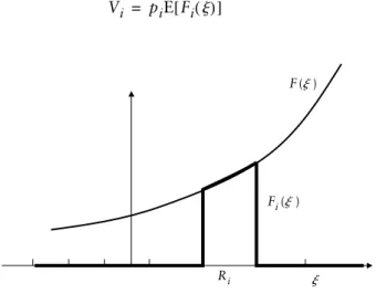
This means that if we buy the jth Arrow-Debreu security in the amount Fj,n(T), we will match the payout of the nth asset in state j. The value of this portfolio is equal to Fs,n(T)s, where s is the value of the sth Arrow-Debreu security.
BASIC DEFINITIONS
This chapter is an attempt to summarize the basics of a complex subject in a way that is accessible to readers with a modest mathematical background. Readers who already have a background in stochastic computation can skip to the next chapter.
PROBABILITY SPACE
Therefore, prior to any observation, information about the true outcome of the price curve is represented by the following set of subsets. The filtration {F0,F1,F2} is created using the first two observations of the up and down movements.
RANDOM VARIABLES
STOCHASTIC PROCESS
The expectation of X depending on the information contained in the - algebra Ft is denoted as follows:. If we assume two -algebras, G and H, such that the information in G is contained in H, then the recurrence expectation of the random variable simplifies to:
WIENER PROCESS
The first variation of a differentiable function is finite while the first variation of the Wiener process is infinite. 2.16). The reason for this will become clear after we discuss the second variant of the Wiener process.
STOCHASTIC INTEGRALS
The Ito integral corresponds to the case where the integrand is evaluated at the beginning of the subintervals used to define the partial sums. These properties of the Ito integral are useful in finding solutions to stochastic differential equations and other applications.
ITO PROCESSES
Covariance of Ito integrals Following similar arguments as in the last section, one can show that the covariance of two Ito integrals is given by
MULTIDIMENSIONAL PROCESSES
As an example, consider a two-dimensional drift-diffusion process, with components X(t) and Y(t) Note that here we have included the coefficients of the linear combination in Equation 2.58 in the definition of. When we deal about multidimensional processes, we will typically favor the vector representation of the Wiener part, shown in Equation 2.64.
ITO’S LEMMA
In this case, two-dimensional processes would be written as 2.69), where X and Y are understood to be vectors, and dW is a vector of uncorrelated Wiener processes. 2.74). Assume a function G(X(t),Y(t),t) of Itov processes. 2.76), where X,Y are vectors, and dW is a vector of uncorrelated Wiener processes.
STOCHASTIC DIFFERENTIAL EQUATIONS
This is one of the earliest Gaussian models for the short interest rate (Ho and Lee 1986). This is so because X(t0) is the initial condition of the solution that determines the behavior of the process at t1≥t0.
MEASURE CHANGES
All we need is reassurance that it is indeed a Wiener process in the measure that made Y(t) a martingale. In the specific case of an expectation that depends on the initial information, we did.
MARTINGALE REPRESENTATION THEOREM
When we apply the Girsanov theorem, we assume that a technical condition called the Novikov condition holds:. 2.139) It is also possible to derive a multidimensional version of the Girsanov theorem, in which case W and are vector processes.
PROCESSES WITH JUMPS
The Poisson model states that the probability of occurrence of one jump in the interval t is ht plus terms of higher order, where h is called the intensity of the jump. Note that the word intensity here refers to the probability of occurrence, not the size of the jump.
ONE-DIMENSIONAL RISK NEUTRAL PRICING
We defined the risk-neutral rate with the condition that the process of the relationship between the price of the underlying asset and the money market account must be a martingale. We put together a portfolio consisting of a certain amount of the underlying asset and a money market account.
MULTIDIMENSIONAL MARKET MODEL
In most cases, the first step to getting the process into the desired benchmark is to get the processes into the risk neutral benchmark. All we have to do is replace the Wiener process in the market benchmark with the Wiener process in the risk neutral benchmark.
THE PRICING EQUATION
The most famous example is the case of the short rate process in the Heath-Jarrow-Morton model (Heath, Jarrow and Morton, 1992). We devote a separate section to the derivation of the price equation in the presence of jumps.
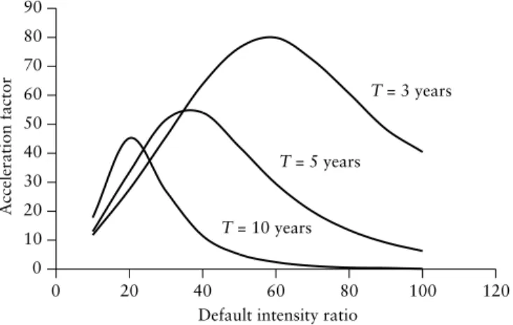
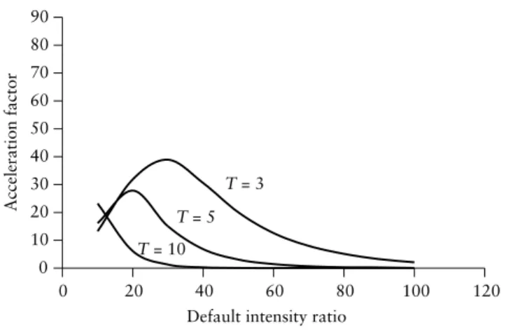
THE PRICING EQUATION IN THE PRESENCE OF JUMPS
For clarity of discussion, assume now that the credit event characterized by x(t) is the default process. How the bond's recovery value is characterized can have a significant impact on the bond's price.
AMERICAN DERIVATIVES
The first condition is that the exercise value and the continuation value of the option are the same at the exercise limit. The second condition is that the gradient of the option value with respect to the underlying variables must be continuous at the exercise limit.
PATH DEPENDENCY
The most important observation is that the value of the option immediately before the sampling time and immediately after the sampling time must be the same. The practical implementation of the continuity condition or shear shock will be discussed in more detail in Chapter 7.
SCENARIO NOMENCLATURE
A dot trajectory can be visualized as a line in the state-versus-time plane, describing the path followed by a realization of the stochastic process (actually by an approximation to the stochastic process). Since this notation is cumbersome, we will abandon it when there is no question of confusion.
SCENARIO CONSTRUCTION
The order of the numerical scheme that characterizes this convergence is called the order of strong convergence. However, when the volatility of the process change is deterministic, the Euler scheme has an order of strong convergence of 1.
BROWNIAN BRIDGE
The Brownian bridge allows you to create that missing part of the trajectories in sets of scenarios without having to reconstruct the trajectories. We can use a Brownian bridge to create a Wiener path and then use the Wiener path to create the trajectory of the process of interest.
JOINT NORMALS BY THE CHOLESKI DECOMPOSITION APPROACH
If the number of observations is insufficient, Choleski decomposition will fail (Choleski decomposition only works with positive definite matrices). If the matrix is invalid due to insufficient precision or because it has been improperly manipulated, this will also be detected by the failure of the Choleski decomposition.
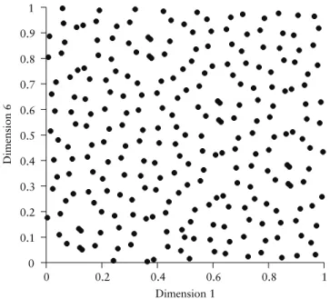
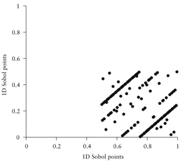
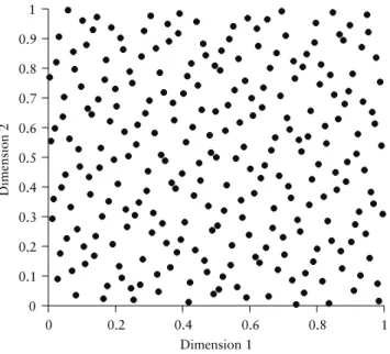
QUASI-RANDOM SEQUENCES
In this case, the speed potential of quasi-random sequences can be more fully realized. As the number of dimensions increases, quasi-random sequences become less and less able to fill space evenly.
INTEREST RATE SCENARIOS
For the construction of the Wiener processes to make sense, all must be expressed to the same extent. To perform the recursive update of the Wiener processes, we can start with any Wi.
PRINCIPAL COMPONENT ANALYSIS TO APPROXIMATE CORRELATION MATRICES
This allows us to take very large integration steps (in the order of 0.5 years for realistic market data) and still map out the path dependence properly. In this chapter we discuss some standard practices and issues related to the pricing of European derivatives.
ROLES OF SIMULATION IN FINANCE
In the case of an option with early exercise, we are interested in (5.2) where is the hold time and F() is the payoff at t. However, since we are only interested in an expectation, we do not necessarily need to perform our simulation on the price measure.
THE WORKFLOW OF PRICING WITH MONTE CARLO
Significance: This refers to the question of whether simulation results can be used for decision making or simply for compliance with regulatory requirements.
ESTIMATORS
This tells us that the standard error of the mean estimator is inversely proportional to the square root of the number of samples. An obvious candidate for estimating the population variance is the sample variance:
SIMULATION EFFICIENCY
This is effectively an application of the Girsanov theorem, where the measure is distorted in such a way that the variance is reduced. Stratification: We arrange the Monte Carlo replications within predetermined regions of the distribution, thus covering the space spanned by the random variables more evenly.
ANTITHETIC VARIATES
Each sampling in a simulation using the antithetical method involves about twice as much work as the Monte Carlo level. The function must be linear in the random variable where the antithetical variable is defined.
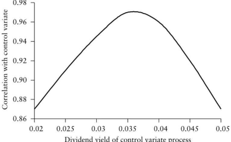
CONTROL VARIATES
Another way to achieve a similar effect is to increase the dividend yield of the underlying control. In this case, the variance of the control variance is approximately 23, and the covariance of the instrument with the control variance is approximately 28.
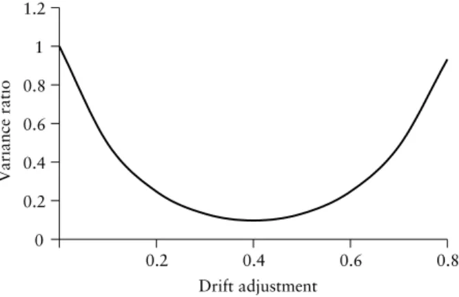
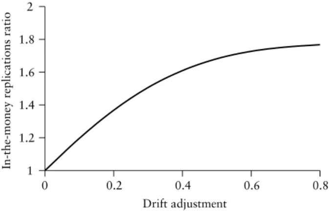
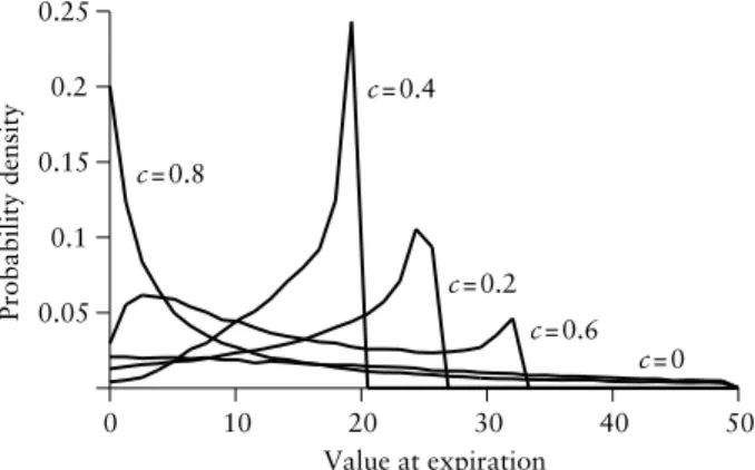
IMPORTANCE SAMPLING
The term in the denominator will reduce the effect of the drift distortion we introduce. The shape of the curve suggests that the countervailing effect of Z(T) is quite symmetrical with the beneficial effect of S(t) in the importance sampling measure.
MOMENT MATCHING
One consequence of this is that we can no longer use the sample variance to determine the standard error. It works by making the properties of the input random variables consistent with the population.
STRATIFICATION
If sample points are assigned according to Equation 5.100, it is easy to verify that the variance of the mean estimator is equal. Another variation would be to use a two-dimensional stratification for the first two dimensions of the Brownian bridge construction (the terminal simulation histogram of standard normals).
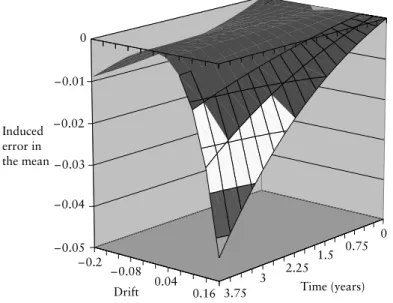
EFFECT OF DISCRETIZATION ON ACCURACY AND THE EMERGENCE OF COMPUTATIONAL BARRIERS
We calculate the errors caused by the discretization in the moments of the log-normal process. This allows us to introduce the discretization error in the representation of the approximate pdf.
THE BASIC DIFFICULTY IN PRICING EARLY EXERCISE WITH SIMULATION
However, when the number of dimensions is three or more, finite differences and other methodologies, such as finite elements, encounter a fundamental problem. When the number of dimensions is large, there are no satisfactory deterministic methods for pricing.
SIMULATION APPLIED TO EARLY EXERCISE
Knowing the exercise policy means that we know the value of the underlying process as a function of the time for which the exercise should occur. One approach is to parameterize the early exercise policy and then find the value of the parameters that maximize the value of the instrument.