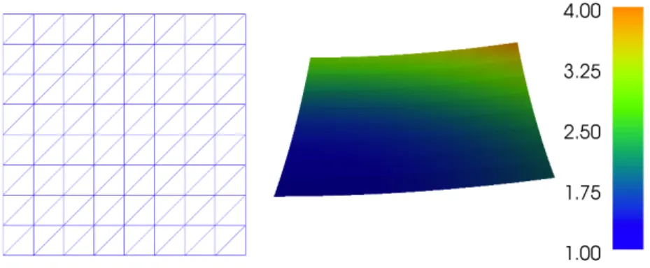
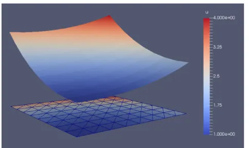
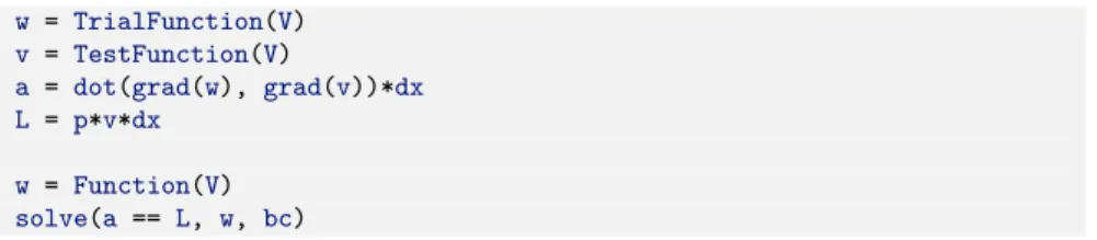
• Tidak ada hasil yang ditemukan

Deflection of a membrane

Our first FEniCS program for the Poisson equation targeted a simple test problem where we could easily verify the implementation. We now turn our attention to a physically more relevant problem with solutions of somewhat more exciting shape.

We want to compute the deflectionD(x, y)of a two-dimensional, circular membrane of radiusR, subject to a loadpover the membrane. The appro- priate PDE model is

T2D=p in ={(x, y)|x2+y2R}. (2.14) Here, T is the tension in the membrane (constant), and p is the external pressure load. The boundary of the membrane has no deflection, implying D= 0as a boundary condition. A localized load can be modeled as a Gaussian function:

p(x, y) = A

2πσexp −1 2

xx0 σ

2

−1 2

yy0 σ

2!

. (2.15) The parameter A is the amplitude of the pressure, (x0, y0)the localization of the maximum point of the load, andσthe “width” of p. We will take the center(x0, y0)of the pressure to be(0, R0)for some0< R0< R.

2.4.1 Scaling the equation

There are many physical parameters in this problem, and we can benefit from grouping them by means of scaling. Let us introduce dimensionless coordinates x¯=x/R, y¯=y/R, and a dimensionless deflection w=D/Dc, where Dc is a characteristic size of the deflection. IntroducingR¯0=R0/R, we obtain

2w

¯x22w

∂y¯2 =αexp −β2x2+ (¯yR¯0)2)

forx¯2+ ¯y2<1, where

α= R2A

2πT Dcσ, β= R

√ 2σ.

With an appropriate scaling, w and its derivatives are of size unity, so the left-hand side of the scaled PDE is about unity in size, while the right-hand side has α as its characteristic size. This suggest choosing α to be unity, or around unity. We shall in this particular case choose α= 4. (One can also find the analytical solution in scaled coordinates and show that the maximum deflectionD(0,0)isDcif we chooseα= 4to determineDc.) With Dc=AR2/(8πσT)and dropping the bars we obtain the scaled problem

− ∇2w= 4 exp −β2(x2+ (yR0)2)

, (2.16)

to be solved over the unit disc with w= 0on the boundary. Now there are only two parameters to vary: the dimensionless extent of the pressure,β, and

the localization of the pressure peak,R0∈[0,1]. As β→0, the solution will approach the special casew= 1−x2y2.

Given a computed scaled solutionw, the physical deflection can be com- puted by

D= AR2 8πσTw .

Just a few modifications are necessary to our previous program to solve this new problem.

2.4.2 Defining the mesh

A mesh over the unit disk can be created by the mshrtool in FEniCS:

from mshr import *

domain = Circle(Point(0, 0), 1) mesh = generate_mesh(domain, 64)

The Circle shape from mshr takes the center and radius of the circle as arguments. The second argument to the generate_mesh function specifies the desired mesh resolution. The cell size will be (approximately) equal to the diameter of the domain divided by the resolution.

2.4.3 Defining the load

The right-hand side pressure function is represented by an Expression ob- ject. There are two physical parameters in the formula for f that enter the expression string and these parameters must have their values set by keyword arguments:

beta = 8 R0 = 0.6

p = Expression(’4*exp(-pow(beta, 2)*(pow(x[0], 2) + pow(x[1] - R0, 2)))’, degree=1, beta=beta, R0=R0)

The coordinates in Expression objects are always an array x with compo- nentsx[0],x[1], and x[2], corresponding tox,y, andz. Otherwise we are free to introduce names of parameters as long as these are given default values by keyword arguments. All the parameters initialized by keyword arguments can at any time have their values modified. For example, we may set

p.beta = 12 p.R0 = 0.3

2.4.4 Defining the variational problem

The variational problem and the boundary conditions are the same as in our first Poisson problem, but we may introduce w instead of uas primary unknown andpinstead of fas right-hand side function:

w = TrialFunction(V) v = TestFunction(V)

a = dot(grad(w), grad(v))*dx L = p*v*dx

w = Function(V) solve(a == L, w, bc)

2.4.5 Plotting the solution

It is of interest to visualize the pressurepalong with the deflectionwso that we may examine the membrane’s response to the pressure. We must then transform the formula (Expression) to a finite element function (Function).

The most natural approach is to construct a finite element function whose degrees of freedom are calculated from p. That is, we interpolate p to the function spaceV:

p = interpolate(p, V)

Note that the assignment to pdestroys the previous Expression objectp, so if it is of interest to still have access to this object, another name must be used for the Functionobject returned by interpolate. The two functions wandpmay be plotted using the built-in plot command:

plot(w, title=’Deflection’) plot(p, title=’Load’)

As before, we also export the solutions in VTK format for visualization in ParaView:

vtkfile_w = File(’poisson_membrane/deflection.pvd’) vtkfile_w << w

vtkfile_p = File(’poisson_membrane/load.pvd’) vtkfile_p << p

Figure 2.3 shows a visualization of the deflection w and the load p created with ParaView.

Fig. 2.3 Plot of the deflection (left) and load (right) for the membrane problem created using ParaView. The plot uses 10 equispaced isolines for the solution values and the optionaljetcolormap.

2.4.6 Making curve plots through the domain

Another way to compare the deflection and the load is to make a curve plot along the linex= 0. This is just a matter of defining a set of points along the y-axis and evaluating the finite element functions wand pat these points:

# Curve plot along x = 0 comparing p and w import numpy as np

import matplotlib.pyplot as plt

tol = 0.001 # avoid hitting points outside the domain y = np.linspace(-1 + tol, 1 - tol, 101)

points = [(0, y_) for y_ in y] # 2D points w_line = np.array([w(point) for point in points]) p_line = np.array([p(point) for point in points]) plt.plot(y, 50*w_line, ’k’, linewidth=2) # magnify w plt.plot(y, p_line, ’b--’, linewidth=2)

plt.grid(True) plt.xlabel(’$y$’)

plt.legend([’Deflection ($\\times 50$)’, ’Load’], loc=’upper left’) plt.savefig(’poisson_membrane/curves.pdf’)

plt.savefig(’poisson_membrane/curves.png’)

This example program can be found in the fileft02_poisson_membrane.py.

The resulting curve plot is shown in Figure 2.4. The localized input (p) is heavily damped and smoothed in the output (w). This reflects a typical property of the Poisson equation.

Fig. 2.4 Plot of the deflection and load for the membrane problem created using Matplotlib and sampling of the two functions along they-axsis.

Open Access This chapter is distributed under the terms of the Creative Commons Attribution 4.0 International License (http://creativecommons.org/licenses/by/4.0/), which permits use, duplication, adaptation, distribution and reproduction in any medium or format, as long as you give appropriate credit to the original author(s) and the source, provide a link to the Creative Commons license and indicate if changes were made.

The images or other third party material in this chapter are included in the work’s Creative Commons license, unless indicated otherwise in the credit line; if such material is not included in the work’s Creative Commons license and the respective action is not permitted by statutory regulation, users will need to obtain permission from the license holder to duplicate, adapt or reproduce the material.

A Gallery of finite element solvers

The goal of this chapter is to demonstrate how a range of important PDEs from science and engineering can be quickly solved with a few lines of FEniCS code.

We start with the heat equation and continue with a nonlinear Poisson equation, the equations for linear elasticity, the Navier–Stokes equations, and finally look at how to solve systems of nonlinear advection–diffusion–reaction equations. These problems illustrate how to solve time-dependent problems, nonlinear problems, vector-valued problems, and systems of PDEs. For each problem, we derive the variational formulation and express the problem in Python in a way that closely resembles the mathematics.