The publisher, the authors and the editors can safely assume that the advice and information in this book is believed to be true and accurate at the date of publication. After digesting the examples in this tutorial, the reader should be able to learn more from the FEniCS documentation, the numerous demo programs that come with the software, and the comprehensive FEniCS book Automated solution of differential equations by the finite element method [26].
The FEniCS Project
What you will learn
Working with this tutorial
Obtaining the software
Installation using Docker containers
2https://www.docker.com. as you run the fenicsproject command) with the FEniCS session. When the FEniCS session starts, it will automatically go into a directory named shared, which will be identical to your current working directory on your host system.
Installation using Ubuntu packages
This means that you can easily edit files and write data within the FENiCS session, and the files will be directly accessible on your host system. It is recommended that you edit your programs with your favorite editor (such as Emacs or Vim) on your host system and use the FEniCS session only to run your program(s).
Testing your installation
Obtaining the tutorial examples
Background knowledge
Programming in Python
All programs in this tutorial are also designed to run under both Python 2 and 3. All print usage in the programs in this tutorial consists of function calls, such as print('a:', a).
The finite element method
Open Access This chapter is distributed under the terms of the Creative Commons Attribution 4.0 International License (http://creativecommons.org/licenses/by/4.0/), which permits use, duplication, adaptation, distribution, and reproduction in any medium or format, provided you give proper credit to the original author(s) and source, link to the Creative Commons license, and indicate whether changes have been made. Images or other third-party material in this chapter are licensed under a Creative Commons Work License unless otherwise noted in the credit line; if such material is not covered by a Creative Commons license for the work and such action is not permitted by law, users will need to obtain permission from the licensee to duplicate, adapt or reproduce the material.
Mathematical problem formulation
Finite element variational formulation
The finite element method for the Poisson equation finds an approximate solution to the variation problem (2.7) by replacing the infinite-dimensional function spaces V and Vˆ with discrete (finite-dimensional) trial and test spaces Vh⊂V and Vˆh⊂Vˆ. Note that the boundary conditions are coded as part of the sample and test space.
Abstract finite element variational formulation
To get (almost) a one-to-one relationship between the mathematical formulation of a problem and the corresponding FENiCS program, we omit the subscript to use for the solution of the discrete problem. We will use for the exact solution of the continuous problem, if we need to make an explicit distinction between the two.
Choosing a test problem
However, if we have a test problem where we know there should be no approximation error, we know that the analytical solution of the PDE problem must be reproduced to machine precision by the program. Typically, elements of degree r can reproduce polynomials of degree r exactly, so this is the starting point for constructing a solution without numerical approximation errors.
FEniCS implementation
The complete program
Running the program
We refer to the Spyder tutorial to learn more about working in the Spyder environment. Run the jupyter notebook command from a terminal window, find the New drop-down menu in the top right corner of the GUI, choose a new notebook in Python 2 or 3, write %load ft01_poisson.py in the empty cell of this notebook, then press Shift+Enter to run the cell.
Dissection of the program
- The important first line
- Generating simple meshes
- Defining the finite element function space
- Defining the trial and test functions
- Defining the boundary conditions
- Defining the source term
- Defining the variational problem
- Forming and solving the linear system
- Plotting the solution using the plot command
- Plotting the solution using ParaView
- Computing the error
- Examining degrees of freedom and vertex values
We also calculate the maximum value of the error at all the vertices of the finite element mesh. However, the degrees of freedom are not necessarily numbered in the same way as the vertices of the mesh.
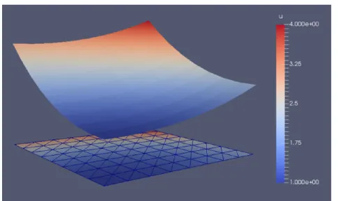
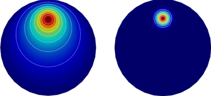
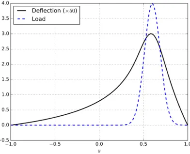
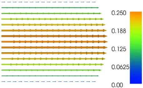
Deflection of a membrane
- Scaling the equation
- Defining the mesh
- Defining the load
- Defining the variational problem
- Plotting the solution
- Making curve plots through the domain
Now there are only two parameters to vary: the dimensionless magnitude of the pressure, β, and . The cell size will be (approximately) equal to the diameter of the domain divided by the resolution.
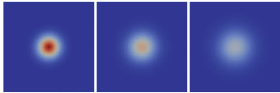
The heat equation
PDE problem
These problems illustrate how to solve time-dependent problems, non-linear problems, vector-valued problems and systems of PDEs. The source functionf and the limit values uD can also vary with space and time.
Variational formulation
Another possibility is to construct only by interpolation of the initial value u0; that is, ifu0=PN. These two strategies are called calculation of the initial state by projection or interpolation.
FEniCS implementation
In the last step of the time loop, we assign the values of the variable u (the new calculated solution) to the variable u_n, which contains the values in the previous time step. To visualize Gaussian hill diffusion, start ParaView, select File–Open.., openheat_gaussian/solution.pvd and click Apply in the Properties pane.
A nonlinear Poisson equation
PDE problem
Once the animation is saved to a file, you can play the animation offline with a player such as mplayer or VLC, or upload your animation to YouTube.
Variational formulation
FEniCS implementation
However, we can use SymPy for symbolic computing and integrate such computations into the FEniCS solver. With 2·(8×8) cells, we reach convergence in eight iterations with a tolerance of 10−9, and the error in the numerical solution is about 10−16.
The equations of linear elasticity
PDE problem
However, when deriving the variation formulation, it is helpful to keep the equations split as above.
Variational formulation
Note that the edge integral on the remaining part ∂Ω\∂ΩT vanishes because of the Dirichlet condition. If we express ∇vas as a sum of its symmetric and anti-symmetric parts, only the symmetric part will survive in the product σ:∇v since σ is a symmetric tensor.
FEniCS implementation
We therefore want the characteristic displacement to be a small fraction of the characteristic length of the geometry. If we take E to be of the same order of magnitude as µ, which is the case for many materials, we realize that γ∼δ−2 is an appropriate choice.
The Navier–Stokes equations
PDE problem
The difference is in the two additional terms %(∂u/∂t+u· ∇u) and the different expression for the stress tensor. The two extra terms express the acceleration which is balanced by the force F=∇ ·σ+f per unit volume in Newton's second law of motion.
Variational formulation
Third, we note that the variational problem (3.32) arises from the integration by parts of the term h−∇ ·σ, vi. By doing so, the remaining boundary term at the outflow becomes spn−µ∇u·n, which is the term appearing in the variational problem (3.32).
FEniCS implementation
We use piecewise quadratic elements for the velocity and piecewise linear elements for the pressure. The next step is to set up the variational form for the first step (3.32) in the solution process.
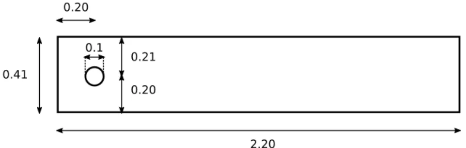
A system of advection–diffusion–reaction equations
PDE problem
We see that the chemical reactions are accounted for in the right side of the PDE system. Moreover, we assume that species A, B and C diffuse through the domain with diffusion (the terms −∇ ·(∇ui)) and are advanced with velocity w (the terms w ∇ui).
Variational formulation
FEniCS implementation
Once the space is created, we need to define our test functions and finite element functions. Since the problem is non-linear, we have to work with functions rather than trial functions for the unknowns.
Combining Dirichlet and Neumann conditions
PDE problem
In this chapter, we take a closer look at how to specify boundary conditions on specific parts (subdomains) of the boundary and how to combine multiple boundary conditions. We will also look at how to generate meshes with subdomains and how to define coefficients with different values in different subdomains.
Variational formulation
FEniCS implementation
Setting multiple Dirichlet conditions
Defining subdomains for different materials
Using expressions to define subdomains
An alternative method is to use a C++ string expression, as we saw earlier, which is much more efficient in FENiCS. However, for more complex subdomains we will have to use a more general technique, as we will see next.
Using mesh functions to define subdomains
Note that the internal function of the Boundary class is (almost) identical to the previous definition of boundary in terms of the boundary function. This will set the mesh function material values to 0 in every cell belonging to Ω0 and 1 in all cells belonging to Ω1.
Using C++ code snippets to define subdomains
This is similar to the Expression subclass we defined above, but we use the member functioneval_cellin instead of the regularevalfunction. In general, however, the definition of subdomains may be available as aMeshFunction (from a data file), perhaps generated as part of the mesh generation process, and not as a simple geometric test.
Setting multiple Dirichlet, Neumann, and Robin conditions
- Three types of boundary conditions
- PDE problem
- Variational formulation
- FEniCS implementation
- Test problem
- Debugging boundary conditions
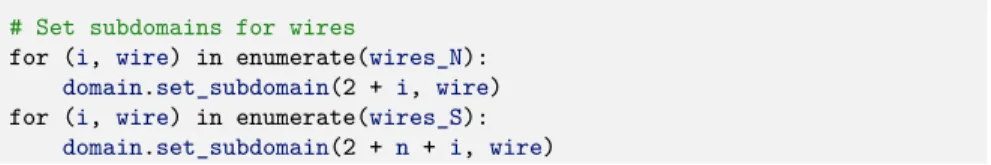
As in Section 4.3, we use the SubDomain subclass to identify different parts of the network function. In the code snippet above, we call an internal method for each grid coordinate.
Generating meshes with subdomains
PDE problem
A static current J= 1 A flows through the copper wires, and we want to calculate the magnetic field B in the iron cylinder, the copper wires and the surrounding vacuum. Once the magnetic vector potential has been calculated, we can calculate the magnetic field B=B(x, y)by.
Variational formulation
FEniCS implementation
The resulting plots of the magnetic vector potential and magnetic field are shown in Figures 4.4 and 4.5. We will also discuss how to use iterative solvers with preconditioners to solve linear systems, how to calculate derivative quantities, such as the flux on part of the boundary, and how to calculate errors and convergence rates.
Refactoring the Poisson solver
- A more general solver function
- Writing the solver as a Python module
- Verification and unit tests
- Parameterizing the number of space dimensions
Mathematically, our unit test is that the finite element solution of our problem whenf=−6 is equal to the exact solution u=uD= 1 +x2+ 2y2 at the vertices of the mesh. Due to rounding errors, we cannot require this error to be zero, but must have a tolerance, which depends on the number of elements and degrees of the polynomials in the finite element basis.
Working with linear solvers
- Choosing a linear solver and preconditioner
- Choosing a linear algebra backend
- Setting solver parameters
- An extended solver function
- A remark regarding unit tests
- List of linear solver methods and preconditioners
Changing a parameter in the global FEniCS parameter database affects all linear solvers (created after the parameter is set). Otherwise, the .config/fenics/dolfin_parameters.xml file in the user's home directory is read, if it exists.
High-level and low-level solver interfaces
Linear variational problem and solver objects
An up-to-date list of available solvers and preconditioners for your FEniCS installation can be prepared by. Thus, changing the value of the tolerance in the global parameter database does not affect the parameters for solvers already created.
Explicit assembly and solve
Then the bc.apply(A, b) call makes the necessary modifications to the linear system to ensure that u is equal to the prescribed limits. Once the linear system is assembled, we must calculate the solution U =A−1b and store the solution U in the vector U = u.vector().
Examining matrix and vector values
Using a non-zero initial guess can be especially important for time-dependent problems or when solving a linear system as part of a nonlinear iteration, as the previous solution vector U will then often be a good initial guess for the solution in the next time step or iteration. In this case, of course, the values in the vectorU are initialized with the previous solution vector (if we just used it to solve a linear system), so the only additional step needed is to set the nonzero_initial_guesstoTrue parameter.
Degrees of freedom and function evaluation
Examining the degrees of freedom
This means we can call coordinates [dof_to_vertex_map(V)] to get an array of all the coordinates in the same order as the degrees of freedom. The following code illustrates how to iterate through all mesh elements and print the coordinates and degrees of freedom associated with the element.
Setting the degrees of freedom
For these elements, we can get the vertex values by calling u.compute_vertex_values(mesh), and we can get the degrees of freedom by calling the callu.vector().array(). To get the coordinates associated with all degrees of freedom, we need to iterate over the elements of the mesh and ask FEniCS to return the coordinates and dofs associated with each element (cell).
Function evaluation
When Lagrange elements are used, this ensures (approximately) that the maximum value of the function is1. The /= operator implies an in-place modification of the object on the left: all elements of the arraynodal_values are divided by the value u_max.
Postprocessing computations
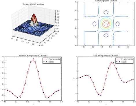
- Test problem
- Flux computations
- Computing functionals
- Computing convergence rates
- Taking advantage of structured mesh data
As we have already seen, the L2 norm of the errorue−u in FEniCS can be implemented by. An implementation of the computation of the convergence rate can be found in the function demo_convergence_rates in the demo program ft10_poisson_extended.py.
Taking the next step