Selection of our books indexed in the Book Citation Index in Web of Science™ Core Collection (BKCI)
Interested in publishing with us?
Contact [email protected]
Numbers displayed above are based on latest data collected.
For more information visit www.intechopen.com Open access books available
Countries delivered to Contributors from top 500 universities
International authors and editors
Our authors are among the
most cited scientists
Downloads
We are IntechOpen,
the world’s leading publisher of Open Access books
Built by scientists, for scientists
12.2%
169,000 185M
TOP 1%
154
6,200
A Global Method for a
Two-Dimensional Cutting Stock Problem in the Manufacturing Industry
Yao-Huei Huang, Hao-Chun Lu, Yun-Cheng Wang, Yu-Fang Chang and Chun-Kai Gao
Abstract
A two-dimensional cutting stock problem (2DCSP) needs to cut a set of given rectangular items from standard-sized rectangular materials with the objective of minimizing the number of materials used. This problem frequently arises in differ- ent manufacturing industries such as glass, wood, paper, plastic, etc. However, the current literatures lack a deterministic method for solving the 2DCSP. However, this study proposes a global method to solve the 2DCSP. It aims to reduce the number of binary variables for the proposed model to speed up the solving time and obtain the optimal solution. Our experiments demonstrate that the proposed
method is superior to current reference methods for solving the 2DCSP.
Keywords:two-dimensional cutting stock problem (2DCSP), rectangular items, optimal solution, deterministic model
1. Introduction
Two-dimensional cutting stock problem (2DCSP) is a well-known problem in the fields of management science and operations research. The problem frequently arises in the manufacturing processes of different products such as wood, glass, paper, steel, etc. In the 2DCSP, a set of given rectangular items is cut from a set of rectangular materials with the aim of determining the minimum number of mate- rials [1, 2]. These applications include sawing plates from wood stocks [3], reel and sheet cutting at a paper mill [4], cutting plates of thin-film-transistor liquid- crystal display (TFT-LCD) from glass substrate [5, 6], placing devices into a system-on-a-chip circuit [7], and container loading or calculation of containers [8, 9]. Minimizing the number of materials is normally the target in this type of the problem because it does not only reduce the overhead consumption but also
enhances environmental protection. The problem in the literatures have been classified as one-dimensional, 1.5-dimensional, and 2DCSPs (Hinxman [10] and Lodi et al. [11]) and suggested two categories of approaches in solving the problems, namely, the heuristic and deterministic approaches (Belov [12], Burke et al. [13], Chen et al. [14], Hopper and Turton [15], Lin [16] and Martello et al. [17]).
Various heuristic approaches have been proposed and discussed in the litera- tures. The primary advantage of this approach is easier in solving the 2DCSP within an acceptable and economical timeframe [18, 19]. The feasible solution is obtained within a reasonable time, while the optimal solution cannot be guaranteed.
Chazelle [20] first proposed a popular heuristic algorithm, called the bottom-left heuristic algorithm. Berkey and Wang [21] proposed a finite best strip heuristic algorithm to improve the original bottom-left method which packs the items directly into the bins with a best-fit policy. On the other hand, Lodi et al. [22]
proposed an integrated heuristic approach that initiates the solution by paralleling the edges of the items and bins (i.e., materials) and utilizes a Tabu search [23, 24]
to explore the neighborhood and refine the possible solution. In order to enhance the effectiveness of the algorithm used, Boschetti and Mingozzi [25, 26] consider empty bins in turn and fill the bins with items in a sequence defined by the prices attributed to the items and update them iteratively. Likewise, Monaci and Toth [27]
initially used Lagrangian-based heuristic to generate a set of covering programming model to obtain a lower bound solution, in which the items cannot be rotated.
They applied geometric analytical techniques and Dantzig-Wolfe decomposition to produce various lower bounds of the 2DCSP so that a better solution can be
compared and obtained [28–31].
Despite the development of heuristic approaches can obtain possible solution in a reasonable time, however there is a scarcity of literature attempting to ensure the achievement of an optimal solution. Moreover, the distance between one random feasible solution and the actual global optimal solution can be enlarged with an increasing problem size. Only a few studies attempted to develop deterministic approaches for an optimal solution. For example, Chen et al. [32] formed a mathe- matical model for packing a set of given rectangular items into a rectangular space in which the dimension of the rectangular space is minimized. The packing problem is equal to the cutting problem, and the problem can also be called as an assortment problem. Moreover, Williams [33] formulated a mathematical model considering the increased generalization of 2DCSP, to solve the problem with various sizes of bins. However, Williams’model contains an excessive number of binary variables as indicated by Pisinger and Sigurd [31] who showed that Williams’model has difficulty in solving a standard 2DCSP by their computational experiments. The subsequent studies by Li and Chang [34], Li et al. [35, 36], Hu et al. [37], and Tsai et al. [38] (these approaches are called Li’s approach in this study) enhanced Chen’s model with reformulation techniques based on reducing binary variables and piecewise linearization technique. The deterministic approaches can guarantee the achievement of global optimization with an acceptable tolerance; however, these approaches are only suitable for the assortment problem (i.e., cutting rectangular items from one material only), while many manufacturing situations require considering minimal number of materials.
Aiming to close the knowledge gap, this study modifies the two programs of the assortment problem proposed by Chen et al. [32] and Li and Chang [34] to be two corresponding deterministic models for the 2DCSP. As an innovative approach, a global approach of the 2DCSP with a logarithmic number of binary variables and extra constraints is proposed and demonstrated.
The remainder of this study is organized as follows: Section 2 discusses the 2DCSP formulations. Section 3 proposes the 2DCSP models with logarithmic number of binary variables and extra constraints. Numerical examples are given in Section 4 to demonstrate the theoretical advances and advantages of the proposed global approach. Section 5 gives the concluding remarks.
2. Problem formulations
Givennsmall rectangular items, the 2DCSP is to cut all items within large rectangular materials with the objective of minimizing the number of materials used. Denotexandyas the width and the length of the enveloping rectangle. By referring to the method of Chen et al. [32], a mathematical program can be formed with the objective of minimizing the volume (i.e., Minxy) as discussed in Section 2.1. In the 2DCSP, the minimal number of materials can reduce the manufacturing costs. Thus Section 2.2 explains how to reformulate two new 2DCSP programs based on the original model in Section 2.1. Firstly, the terminologies, including decision variables and parameters, are introduced inTables 1and2.
2.1 Cutting problem in one material
The cutting problem considering one material is also called the assortment problem, which considers cutting a set of given rectangular items within a rectan- gular material of minimum area. Avoiding the overlapping of items is the core requirements. Chen et al. [32] and Li and Chang [34] use four binary variables
ai,j,bi,j,ci,j,di,j
and two binary variablesui,j,vi,j
, respectively, to handle the non-overlapping conditions, as shown inTable 3.
The following assortment program is proposed by Chen et al. [32]:
Original (a) Minxy
s:t:xjþpjsjþqj1sj
≤xiþx1ai,j
fori, j¼1,…,nandi<j, (1)
Parameter Meaning
n The number of given rectangular items needed to be cut m The number of rectangular materials with the same size
pi,qi
The width and length of given rectangular itemifori¼1,…,n x,y
ð Þ xandyare the upper bounds ofxandy, respectively. These items also denote the width and length of a given rectangular material
Table 1.
Parameters in the 2DCSP.
Variable Meaning xi,yi
The bottom-left coordinate of rectangular itemi x,y
ð Þ The top-right coordinate of the rectangular material ai,j,bi,j,ci,j,di,j
A set of binary variables expressing the non-overlapping conditions for a pair of rectangular itemsi and rectangular itemsjfori<j, which are defined by Chen et al. [32]
ui,j,vi,j
A pair of binary variables expressing the non-overlapping conditions for a pair of rectangular items iand rectangular itemsjfori<j, which are defined by Li and Chan [34]
si An orientation indicator for a given rectangular itemi.si¼1 ifpiis parallel to thex-axis; otherwise, si¼0 ifpiis parallel to they-axis (siis a binary variable)
Y The accumulated length of all materials used.
Table 2.
Decision variables in the 2DCSP.
xiþpisiþqið1siÞ≤xjþx1bi,j
fori,j¼1,…,nandi<j, (2) yjþqjsj þpj1sj
≤yiþy1ci,j
fori,j¼1,…,nandi<j, (3) yiþqisiþpið1siÞ≤yjþy1di,j
fori, j¼1,…,nandi<j, (4) ai,jþbi,jþci,jþdi,j ¼1 fori, j¼1,…,nandi<j, (5) xiþpisiþqið1siÞ≤x≤xfori ¼1,…,n, (6) yiþqisiþpið1siÞ≤y≤yfori¼1,…,n, (7) whereai,j,bi,j,ci,j,di,j, andsiare binary variables; xiandyiare nonnegative continuous variables; Constraints (1)–(5) ensure that the rectangular items are non- overlapping, and Constraints (6) and (7) are to cut all of the rectangular items within an enveloping rectangular materialðx,yÞ.
Remark 1.Original (a) uses 2n2nbinary variables (ai,j,bi,j,ci,j,di,j) and 2:5n n1
ð Þ þ2nconstraints to formulate an assortment problem withnrectangular items.
By referring to Li and Chang [34], an alternative mathematical model can be expressed as follows:
Original (b) Minxy
s.t.(6) and (7),
xjþpjsjþqj1sj
≤xiþx u i,jþvi,j
fori, j¼1,…,nandi<j, (8) xiþpisiþqið1siÞ≤xjþx 1ui,jþvi,j
fori, j¼1,…,nandi<j, (9) yjþqjsjþpj1sj
≤yiþy 1þui,jvi,j
fori, j¼1,…,nandi< j, (10) yiþqisiþpið1siÞ≤yjþy2ui,jvi,j
fori,j¼1,…,nandi<j, (11) whereui,j,vi,j, andsiare binary variables;xiandyiare nonnegative continuous variables; and Constraints (8)–(11) ensure that the rectangular items are non-overlapping.
Remark 2.Original (b) usesn2 binary variables (ui,j,vi,j) and 2n2 constraints to formulate an assortment problem withnrectangular items.
However, these two models are inappropriate for directly solving the general 2DCSP because the objective of the 2DCSP must minimize the number of materials used for cutting all items. By referring to the two models above, two corresponding 2DCSP models are proposed in Section 2.2.
Method Chen et al. [32] Li and Chang [34] Condition
Case ai,j bi,j ci,j di,j ui,j ui,j
1 1 0 0 0 0 0
2 0 1 0 0 1 0
3 0 0 1 0 0 1
4 0 0 0 1 1 1
Table 3.
Four cases of non-overlapping conditions.
2.2 General deterministic models of 2DCSP
As mentioned above, we need to find out the minimal number of materials used for cutting all items. Original (a) is then reformulated as a general
deterministic model of 2DCSP, where cuttingnrectangular items frommmaterials, as shown in P1 (a):
P1 (a) MinY
s.t.(1), (2) and (5) in Original (a), yjþqjsjþpj1sj
≤yiþmy1ci,j
fori, j¼1,…,nandi<j, (12) yiþqisiþpið1siÞ≤yj þmy 1di,j
fori, j¼1,…,nandi< j, (13) xiþpisiþqið1siÞ≤xfori¼1,…,n, (14) yiþqisiþpið1siÞ≤ Xm
k¼1
kyQi,k fori¼1,…,n, (15)
yi≥ Xm
k¼1
k1
ð ÞyQi,kfori¼1,…,n, (16)
Xm
k¼1
Qi,k ¼1 fori¼1,…,n, (17) yiþqisiþpið1siÞ≤Y fori ¼1,…,n, (18) wheresi,ai,j,bi,j,ci,j,di,j, andQi,k are binary variables;xi,yi andY are nonnega- tive continuous variables; Constraints (1), (2), (5), (12) and (13) ensure that the rectangular items are non-overlapping; Constraints (15)–(17) mean that each rect- angular item is fitly cut from one of themmaterials; Constraint (18) obtains the accumulated length of materials used; and the objective function minimizes the accumulated length of materials used.
There arenmnew binary variables (i.e.,Qi,k fori¼1, 2,…,nandk¼1, 2,…,m) in Constraints (15)–(17) of P1 (a) model. It aims to cut theith rectangular item from thekth material ifQi,k ¼1, and Constraint (17) forces any rectangular item to be cut from one of such materials. Supposing that rectangular itemi0 is cut from the k0th material, thenQi0,k0 ¼1 andQi0,k ¼0 fork6¼k0 andk¼1, 2,…,m. Constraints (15)–(17) will force they-axis position of rectangular itemi0 cut from thek0th material as shown below:
yi0 þqi0si0 þpi0ð1si0Þ≤k0y, (19) k01
y≤yi0: (20)
Remark 3.P1 (a) requires 2n2nð1mÞbinary variables and 5nð 2þ3nÞ=2 constraints to form a 2DCSP program.
Referring to the Original (b), another corresponding 2DCSP program can be formulated as follows:
P1 (b) Min Y
s.t.(8), (9), (14)–(18), yjþqjsjþpj1sj
≤yiþmy1þui,jvi,j
fori, j¼1,…,nandi< j, (21)
yiþqisiþpið1siÞ≤yjþmy2ui,jvi,j
fori, j¼1,…,nandi< j, (22) where si,ui,j,vi,j, andQi,k are binary variables andxi,yi, andY are nonnegative continuous variables.
Remark 4.P1 (b) requiresn2þnmbinary variables and 2n nð þ1Þconstraints to formulate a 2DCSP program.
Although both P1 (a) and P1 (b) can obtain a minimal number of materials used, there is mainly an issue needed to be addressed. That is, an excessive number of binary variablesQi,k is used to assign rectangular itemiinto one of the materials;
such that the computational load becomes a serious burden as the size of the problem grows.
As indicated by Li et al. [39], reducing the number of binary variables can accelerate the solving speed. Hence, we can roughly estimate the number of mate- rials by the following remark.
Remark 5.The number of materials can be reduced frommtof wheref≤mby the following initial calculating:
f ffi⌈Pn
i¼1
xiyi=xy⌉, (23)
where iff value is not big enough, i.e., in solving P1(a) and P1(b) are infeasible, then we can accumulatef, i.e.,f ¼f þ1, until feasible solutions exist.
By referring to Remark 5, the number of binary variables in Constraints (15)–(18) can be reduced fromnmto nf wheref≤m. Moreover, this study
proposes a reformulation technique using logarithmic number of binary variables for the P1 (a) and P1 (b) models. The detail of technique is then discussed in Section 3.
3. Logarithmic reformulation technique of 2DCSP
After considering Remark 5, for a 2DCSP withnrectangular items andf mate- rials, the P1 (a) and P1 (b) models will requirenf binary variables (Qi,k) to cut each rectangular item from one of the materials. The computational efficiency of the P1 (a) and P1 (b) models become a serious burden when an increasing size of the 2DCSP. For any rectangular itemi, Constraint (17) (Pf
k¼1Qi,k ¼1) is an SOS1 constraint [40], which is an ordered set of variables where only one variable may be one. An SOS1 constraint model with sizef will generally requiref binary variables.
However, Vielma and Nemhauser [41] use SOS1 constraint with a logarithmic number of binary variables and constraints. This section utilizes the concept of Vielma and Nemhauser [41] and introduces the binary variablesQi,r(i¼1,…,nand r¼1,…,⌈log2f⌉) to replace the original binary variables (Qi,k) of the P1 (a) and P1 (b) models. Thus, the number of required binary variables can be reduced fromnf ton⌈log2f⌉. The following remarks and propositions discuss the logarithmic reformulation technique of the 2DCSP.
Remark 6.LetK ¼1, 2,…,f ¼2θ
,θ¼⌈log2f⌉, andk∈K be the injective function forB:1, 2,…, 2θ
!f0, 1gθ, which can be expressed as follows:
B kð Þ ¼½w1,w2,…,wθT andwr ¼1 ⌈ k 2r1⌉%2
forr¼1,…,θ: (24) Proposition 1.LetK ¼f1,…,fg,θ¼⌈log2f⌉andk∈K; the original SOS1 Constraint in (25) which requiresf binary variablesðQkÞcan be replaced by the Constraint set (26) and (27):
X
f
k¼1
Qk ¼1 andQk∈f0, 1g: (25)
The Constraint set (25) and (26) only requiresθbinary variablesðQrÞ, 2θ additional constraints, andf additional continuous variablesð Þ:λk
X
f k¼1
λk ¼1, (26)
X
k∈Sþð Þr
λk ¼Qrforr¼1,…,θ, (27)
where
i.Qr∈f0, 1g.
ii.B kð Þis an injective function based on Remark 6 (i.e.,B kð Þ ¼½w1,w2,…,wθT withwr∈f0, 1gforr¼1,…,θ).
iii.Sþð Þ ¼r fk∈Kj∀B kð Þwhere wr ¼1gandSð Þ ¼r fk∈Kj∀B kð Þwhere wr¼0g.
Proof:Following Li et al. [39], Constraints (26) and (27) are used to construct the SOS1 property.
Following Proposition 1, we then have Proposition 2 that uses⌈log2f⌉binary variables to determine whether rectangular itemicould be exactly cut from one of the given materials.
Proposition 2.Letf be the number of materials,ythe length of material, and yithe y-axis position of rectangular itemi. The original Constraint set (15)–(17) of the P1 (a) and P1 (b) models will be re-expressed by the following
linear system, which holds the rectangular itemito be cut from one of the given materials:
yiþqisiþpið1siÞ≤ X
f
k¼1
kyλi,kfori¼1,…,n, (28)
yi≥ Xf
k¼1
k1
ð Þyλi,k fori ¼1,…,n, (29)
X
f
k¼1
λi,k ¼1 fori¼1,…,n, (30) X
k∈Sþð Þr
λi,k ¼Qi,r fori¼1,…,nandr¼1,…,θ¼⌈log2 f⌉, (31)
whereSþð Þr andSð Þr are the same as the notations in Proposition 1 and si,Qi,r∈f0, 1g.
Proof:According to Proposition 1, the continuous variablesλi,k with the
Constraint set (30) and (31) have the characteristics of binary variables. Therefore, the Constraint set (28)–(30) is equivalent to the Constraint set (15)–(17).
Two types of 2DCSP models are formulated by utilizing Proposition 2 as the following P2 (a) and P2 (b), respectively:
P2 (a) Min Y
s.t.(1), (2), (5), (12)–(14), (18) and (28)–(31),
whereY,xi,yi,λi,k≥0 andai,j,bi,j,ci,j,di,j,si,Qi,r∈f0, 1gfori, j¼1,…,n,i<j, k¼1,…,f, andr¼1, 2,…⌈log2f⌉.
Remark 7.P2 (a) requiresn2nþ⌈log2f⌉1
binary variables and 5n2þ10nþ
⌈log2f⌉constraints to express a 2DCSP model.
P2 (b) Min Y
s.t.(8), (9), (14), (18), (28)–(31),
whereY,xi,yi,λi,k≥0 and si,ui,j,vi,j,Qi,r∈f0, 1gfori,j¼1,…,n,i< j,k¼ 1,…,f andr¼1,…,⌈log2f⌉.
Remark 8.P2 (b) requiresn n þ⌈log2f⌉
binary variables and n2nþ2⌈log2 f⌉þ3
constraints to express another 2DCSP model.
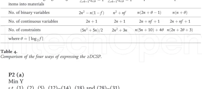
Table 4shows a comparison of the four ways of expressing the 2DCSP, and it clearly lists the number of binary variables, auxiliary continuous variables, and constraints.
4. Numerical examples
There are two examples modified from Tsai et al. [38]. The detail sizes of rectangular items and materials are listed inTable 5. We implement a Java pro- gram, which embedded an optimization package GUROBI (2011) as an MIP solver
Items P1(a) P1(b) P2(a) P2(b)
Concept of non-overlapping Chen et al.
[32]
Li and Chang [34]
Chen et al. [32] Li and Chang [34]
Constraints for assigning rectangular items into materials
Pf
k¼1Qi,k¼1 Pf
k¼1Qi,k¼1 Proposition 2 Proposition 2
No. of binary variables 2n2nð1fÞ n2þnf nð2nþθ1Þ n nð þθÞ No. of continuous variables 2nþ1 2nþ1 2nþnf þ1 2nþnfþ1 No. of constraints ð5n2þ5nÞ=2 2n2þ3n nð5nþ10Þ þ4θ nð2nþ2θþ3Þ whereθ¼⌈log2f⌉
Table 4.
Comparison of the four ways of expressing the 2DCSP.
Problem Size of material
Qty. of items
f Size of items (pi,qi)
1 (40, 69) 8 2 (25, 20), (16, 20), (15, 20), (14, 20), (20, 18), (15, 17), (30, 16), (30, 14)
2 (25, 150) 12 2 (32, 24), (26, 20), (25, 20), (24, 20), (40, 18), (35, 17), (20, 16), (18, 16), (38, 15), (50, 15), (18, 4), (25, 5)
Table 5.
Sizes of rectangular items and materials.
for solving the two examples with the four proposed models (P1 (a), P1 (b), P2 (a), P2 (b)). The experimental tests were run on a PC equipped with an Intel® Core™
2 Duo CPU, 4GB RAM, and 32 bit Windows 7 operating system.
The two problems with the number of materials firstly estimated to be 2 (i.e., f ¼2) are solved by using the four models including P1(a), P1(b), P2(a), and P2 (b).Table 6shows the experiment results of two problems. Both ofFigures 1and2 depict the visualization solutions. In solving four models, we obtain the same objective values of (83) and (293) in Problem 1 and Problem 2, respectively. The results clearly indicate that solving P2(a) and P2(b) is much more
computationally efficient than that of P1(a) and P1(b). By observing the four models, we know that both P2(a) and P2(b) use proposed approach to reduce the numbers of binary variables. The results demonstrate that the adoption of a smaller number of binary variables can enhance the solving efficiency in
solving 2DCSP.
Items P1 (a) P1 (b) P2 (a) P2 (b)
Problem 2 Y= 83
No. of 0–1 variables 136 80 128 72
No. of cont. variables 17 17 33 33
No. of constraints 180 152 404 168
Iterations 621,821 686,982 263,296 293,432
Nodes 176,776 211,564 70,154 111,173
Solving time 18.8 18.0 7.5 9.1
Problem 2 Objective = 293
No. of 0–1 variables 300 168 288 156
No. of cont. variables 25 25 49 49
No. of constraints 390 324 844 348
Iterations 31,166,357 1,017,922 1,114,911 805,136
Nodes 9,766,654 244,444 266,672 229,701
Solving time 856.5 24.5 34.9 19.4
Table 6.
Experiment results of two problems.
Figure 1.
Visualization result of Example 1.
5. Conclusions
This study develops a logarithmic reformulation technique for reducing the required binary variables of the mixed integer program for two-dimensional cutting stock problem in the manufacturing industry. A reformulated logarithmic tech- nique in the deterministic method reduces the number of binary variables to speed up the solving time. The deterministic methods are guaranteed to find a global optimal solution, but the computational complexity grows rapidly by increasing the number of variables and constraints. Future studies are suggested to enhance the computational efficiency for globally solving large-scale 2DCSP, such as column generation, cloud computing and meta-heuristic algorithms.
Author details
Yao-Huei Huang*, Hao-Chun Lu, Yun-Cheng Wang, Yu-Fang Chang and Chun-Kai Gao
Department of Information Management, College of Management, Fu Jen Catholic University, Taipei, Taiwan
*Address all correspondence to: [email protected]
© 2020 The Author(s). Licensee IntechOpen. This chapter is distributed under the terms of the Creative Commons Attribution License (http://creativecommons.org/licenses/
by/3.0), which permits unrestricted use, distribution, and reproduction in any medium, provided the original work is properly cited.
Figure 2.
Visualization result of Example 2.
References
[1]Dyckhoff H. A typology of cutting and packing problems. European Journal of Operational Research. 1990;
44:145-159
[2]Wäscher G, Hauβner H,
Schumann H. An improved typology of cutting and packing problems.
European Journal of Operational Research. 2007;183:1109-1130 [3]Reinders MP. Cutting stock optimization and integral production planning for centralized wood
processing. Mathematical and Computer Modelling. 1992;16:37-55
[4]Correia MH, Oliveira JF, Ferreira JS.
Reel and sheet cutting at a paper mill.
Computers and Operations Research.
2004;21:1223-1243
[5]Tsai JF, Hsieh PL, Huang YH. An optimization algorithm for cutting stock problems in the TFT-LCD industry.
Computers and Industrial Engineering.
2009;57:913-919
[6]Lu HC, Huang YH, Tseng KA. An integrated algorithm for cutting stock problems in the thin-film transistor liquid crystal display industry.
Computers and Industrial Engineering.
2013;64:1084-1092
[7]Lim SK. Physical design for 3D system on package. IEEE Design and Test of Computers. 2005;22:532-539 [8]Pisinger D. Heuristics for the container loading problem. European Journal of Operational Research. 2002;
141:382-392
[9]Wang Z, Li KW, Levy JK. A heuristic for the container loading problem: A tertiary-tree-based dynamic space decomposition approach. European Journal of Operational Research. 2008;
191:86-99
[10]Hinxman AI. The trim-loss and assortment problem: A survey.
European Journal of Operational Research. 1980;5:8-18
[11]Lodi SM, Vigo D. Recent advances on two-dimensional bin packing problems. Discrete Applied Mathematics. 2002;123:379-396 [12]Belov G. Problems, Models and Algorithms in One- and Two-
Dimensional Cutting [Ph.D. Thesis].
Technischen University Dresden; 2003 [13]Burke EK, Kendall G, Whitewell G.
A new placement heuristic for the orthogonal stock-cutting problem.
Operations Research. 2004;52:655-671 [14]Chen CS, Lee SM, Shen QS. An analytical model for the container loading problem. European Journal of Operational Research. 1995;80:68-76 [15]Hopper E, Turton B. A genetic algorithm for a 2D industrial packing problem. Computers and Industrial Engineering. 1999;37:375-378
[16]Lin CC. A genetic algorithm for solving the two-dimensional assortment problem. Computers and Industrial Engineering. 2006;50:175-184
[17]Martello S, Pisinger D, Vigo D. The three-dimensional bin packing problem.
Operations Research. 2000;48:256-267 [18]Jakobs S. On genetic algorithms for the packing of polygons. European Journal of Operational Research. 1996;
88:165-181
[19]Leung TW, Chan CK, Troutt MD.
Application of a mixed simulated annealing-genetic algorithm for a 2D packing problem. European Journal of Operational Research. 2003;145:530-542
[20]Chazelle B. The bottom-left bin- packing heuristic: An efficient implementation, computers. IEEE Transactions on Computers. 1983;100:
697-707
[21]Berkey JO, Wang PY. Two- dimensional finite bin-packing
algorithms. Journal of the Operational Research Society. 1987;38:423-429 [22]Lodi SM, Vigo D. Heuristic and metaheuristic approaches for a class of two-dimensional bin packing problems.
INFORMS Journal of Computing. 1999;
11:345-357
[23]Glover F, McMillan C. The general employee scheduling problem: An integration of MS and AI. Computers and Operations Research. 1986;13:
563-573
[24]Glover F, Laguna M. Tabu Search.
Boston: Kluwer Academic Publishers;
1997
[25]Boschetti MA, Mingozzi A. The two- dimensional finite bin packing problem.
Part I: New lower bounds for the oriented case, 4OR-Q. Journal of the Operational Research Society. 2003a;1:
274-294
[26]Boschetti MA, Mingozzi A. The two-dimensional finite bin packing problem. Part II: New lower and upper bounds, 4OR: 4OR-Q. Journal of the Operational Research Society. 2003b;1:
135-147
[27]Monaci M, Toth P. A set-covering- based heuristic approach for bin-
packing problems. INFORMS Journal of Computing. 2006;18:71-85
[28]Dell’Amico M, Martello S, Vigo D. A lower bound for the non-oriented two- dimensional bin packing problem.
Discrete Applied Mathematics. 2002;
118:13-24
[29]Fekete SP, Schepers J. New classes of lower bounds for the bin packing
problem. Mathematical Programming.
2001;91:11-31
[30]Martello S, Vigo D. Exact solution of the two-dimensional finite bin packing problem. Management Science. 1998;
44:388-399
[31]Pisinger D, Sigurd M. The two- dimensional bin packing problem with variable bin sizes and cost. Discrete Optimization. 2005;2:154-167 [32]Chen CS, Sarin S,
Balasubramanian R. A mixed-integer programming model for a class of assortment problems. European Journal of Operational Research. 1993;65:
362-367
[33]Williams HP. Model Building in Mathematical Programming. fourth ed.
Chichester: Wiley; 1999
[34]Li HL, Chang CT. An approximately global optimization method for
assortment problems. European Journal of Operational Research. 1998;105:
604-612
[35]Li HL, Chang CT, Tsai JF.
Approximately global optimization for assortment problems using piecewise linearization techniques. European Journal of Operational Research. 2002;
140:584-589
[36]Li HL, Tsai JF, Hu NZ. A distributed global optimization method for packing problems. The Journal of the
Operational Research Society. 2003;54:
419-425
[37]Hu NZ, Tsai JF, Li HL. A global optimization method for packing problems. Journal of the Chinese Institute of Industrial Engineers. 2002;
19:75-82
[38]Tsai JF, Wang PC, Lin MH. An efficient deterministic optimization approach for rectangular packing problems. Optimization. 2013;62:
989-1002
[39]Li HL, Huang YH, Fang SC. A logarithmic method for reducing binary variables and inequality constraints in solving task assignment problems.
INFORMS Journal of Computing. 2013;
25(4):643-653
[40]Beale EML, Forrest JJH. Global optimization using special ordered sets.
Mathematical Programming: Series A and B. 1976;10:52-69
[41]Vielma JP, Nemhauser G. Modeling disjunctive constraints with a
logarithmic number of binary variables and constraints. Mathematical
Programming. 2011;128:49-72
Selection of our books indexed in the Book Citation Index in Web of Science™ Core Collection (BKCI)
Interested in publishing with us?
Contact [email protected]
Numbers displayed above are based on latest data collected.
For more information visit www.intechopen.com Open access books available
Countries delivered to Contributors from top 500 universities
International authors and editors
Our authors are among the
most cited scientists
Downloads
We are IntechOpen,
the world’s leading publisher of Open Access books
Built by scientists, for scientists
12.2%
169,000 185M
TOP 1%
154
6,200
Selection of Food Items for Diet Problem Using a Multi-objective Approach under Uncertainty
Saman Hassanzadeh Amin, Samantha Mulligan-Gow and Guoqing Zhang
Abstract
It is a problem that concerns us all: what should we eat on a day-to-day basis to meet our health goals? Scientists have been utilizing mathematical programming to answer this question. Through the use of operations research techniques, it is possible to find a list of foods that, in a certain quantity, can provide all nutrient recommendations in a day. In this research, a multi-objective programming model is provided to determine the selected food items for a diet problem. Two solution approaches are developed to solve this problem including weighted-sums and ε-constraint methods. Two sources of uncertainty have been considered in the model. To handle these sources, a scenario-based approach is utilized. The applica- tion of this model is shown using a case study in Canada. Using the proposed model and the solution approaches, the best food items can be selected and purchased to minimize the total cost and maximize health.
Keywords:food optimization, diet, nutrition, multi-objective programming, uncertainty
1. Introduction
It is common knowledge that diet affects general health in extraordinary ways.
What is less clear is what specific diet results in the best health. Some diets restrict the quantity of carbohydrates or fats, others require particular percentages of the three macronutrients (carbohydrates, fats, and protein), some depend solely on liquids, and the list continues [1–5]. There are unlimited amounts of unique diets being used today by people all over the world, especially since countless health trends have become the new normal. One thing that can be agreed upon is the recommended dietary allowances (RDA), given by the federal government of Canada, which presents the quantity of vitamins and nutrients needed to meet requirements. So it is important to determine the combination of the seemingly infinite food items that reaches nutrient goals in the most efficient manner.
The diet problem was first introduced by Stigler [6] as a way to determine the minimum cost of feeding an adult for a year. Many models have since explored diet optimization with the objectives of reaching recommended nutrient levels while keeping the diets similar to actual intakes, decreasing environmental impact, or satisfying taste. There are numerous models that can be used to create unique diets
based on the main target criteria. These models include linear and nonlinear, multi- objective, goal-oriented, integer, and mixed-integer programming. Each yields spe- cific results due to the mathematical basis.
2. Literature review
In this section, some related papers are discussed, classified on the subject of the model’s goal. Most research of the diet problem is centered on at least one of the following targets: cost of diet, similarity of diet, environmental sustainability of diet, prevention of health implications by diet, and taste/satisfaction of diet.
2.1 Cost of diet
The first diet problem [6] focused on minimizing the cost of food. The author showed that to feed one man for a year can cost as little as $39.93 (1939 prices).
Certainly, lowering the grocery bill is a desire for all and this type of objective is quite common to this day. One paper discusses whether it is too expensive to follow a healthy diet, comparing 2012 and 1980 costs [7]. Stigler’s problem was reinvented with updated costs and nutritional information in 1999 [8] and taste of diet was included in the cost minimization by Smith [9].
In recent years, further papers focused on more specific problem statements and how they are affected by expense. In Mozambique, the affordability of a nutritious meal plan was studied and fortified foods were assessed with the hopes of creating more economic value [10]. Specific diets have also been studied to determine whether they can be accomplished in a cost-effective manner [11]. To attempt a solution of high-cost food, James David Ward studied urban agriculture and how it could reduce grocery expenses [12].
2.2 Sustainability of diet
Considering that livestock production is a major contributor to greenhouse gas emissions, worldwide [13], the question of nutritional sustainability has been asked and answered. Multi-objective linear programming was used to formulate three unique diets that minimized cost, environmental indicators (H2O use, amount of land to regenerate the resources, and CO2emissions), and the integration of the two [13]. Another study was completed in which the optimal diet was to be as similar to the general, observed diet [14]. This chapter noted that a sustainable diet reduces greenhouse gas emissions by 27% [14]. Mathematical programming was also used to study which food sources contributed least to environmental footprints such as land use, carbon and nitrogen footprints [15]. Barre et al. [16] found diets by using–on the reduction percentage of environmental impacts being at least 30%. It was concluded that all diets required a decrease in meat consumption to meet the sustainability factors [16]. The cost of feeding cattle was found to increase (by as much as 48.5%) in a hypothetical scenario where there was either a tax on green- house gas emissions or a constraint on methane emissions applied [17].
2.3 Disease prevention of diet
It is commonly known that what you eat affects your health. Studies have been conducted to explain how diets can reduce your risk of certain health risks and concerns. Observed diets and those recommended by the World Cancer Fund and the American Institute of Cancer Research were compared by Masset et al. [18].
Furthermore, obesity and its relation to dietary intake has been a frequent topic of interest. Silva et al. [19] presented the possibility of a diet that constricts amount of calories by increasing the quantity of proteins eaten in a day, which will then create the opportunity for weight loss.
2.4 Similarity of diet
In many papers, one of the objectives (usually secondary) is to minimize the difference between the proposed diet and the current, observed diet of a group of people being studied [16, 20–23]. This is done for many reasons: to ensure palat- ability, ease of acceptance, and culturally appropriate solutions. This focus is often the backbone of the programming calculation as it guarantees a certain level of logic and reality.
InTable 1, related papers are organized by which mathematical programming approach was utilized. Linear programming (LP) is used for optimizing (maximiz- ing or minimizing) a linear function of many variables [24], while nonlinear pro- gramming (NLP) does the same when there is(are) one or more nonlinear functions in the problem [25, 26]. For computing problems with multiple objectives, goal programming (GP) is often used [27]. This technique is popular in recent diet studies due to its potential ability to achieve a more realistic food balance [28].
Linear programming has been seen inTable 1as the most commonly used tech- nique for diet problems, including a paper done to disavow goal programming [29].
Table 1.
Review of some related papers and their operations research techniques [32–34].
Multi-objective programming (MOP) is used when there are multiple, competing objectives that result in more than one optimal solution [30]. With uncertain environments, fuzzy set theory (FST) and some specific techniques can be applied so that qualitative statements can be described numerically without losing
precision [31].
Included inTable 1is the format of the results in each respective paper. Some papers explicitly create day-to-day diets, including exact foods and their quantities.
We call them“Final Diet.”Other papers note the nutrients that their proposed model offers if created into a diet. These are called“Nutrients”inTable 1. Other papers only present the model that is used to create a diet without stating which foods should be chosen. In these papers, no specific food intake is specified, rather only the math is presented.
2.5 Research gaps
There are some gaps in the literature of diet problems. There are a few papers in the literature that have considered multiple objectives in diet problems. Among them, most publications have focused on two objectives. Therefore, the research gap can be filled by considering more than two objectives. The other point is related to the availability of data. In recent years, companies have been forces to provide nutritional information for the packages and products. Therefore, a lot of useful information is available that is new and valuable in this field. Case studies can be conducted based on the available information. The other gap in the literature is about the uncertainty of the parameters in diet problems. Most of the papers in this area have ignored uncertain parameters and their effects on the results.
2.6 Research contributions
The main research contributions of this paper are defined in this section.
• A novel optimization model is provided to determine personal food selection.
• Multiple objectives are considered in the mathematical model. To our
knowledge, these objectives have not been considered simultaneously in the other papers in the literature.
• The mathematical formulation is solved by two solution approaches including weighted-sums andε-constraint approaches. As a result, the efficient solutions are obtained.
• Uncertainty in the parameters is considered using an effective scenario-based solution approach. Different combinations of the scenarios are analyzed in this paper.
• The application of the model is shown using real data and a case study in Canada.
3. Problem statement
As discussed previously, the optimization of diets is a continuously important problem since we all eat every day. What is more, the food costs money and affects our health and well-being. Some diseases related to obesity (e.g., cardiovascular and
diabetes) have significant impacts in Canada. Some factors of diets such as sugars, sodium, and fat play important roles on health of people. A study done by Hajizadeh et al. [35] found that body mass index, an indicator of obesity, is negatively related to household income (and fruit and vegetable consumption). Families across Can- ada suffer from food poverty: the inability to purchase healthy, nutritious food for their loved ones [36]. There are people who have to make the difficult decision to either pay rent, or buy groceries. These people should be able to know that what money they put toward food is being used in the most efficient way possible. On the other hand, if food can be used to combat major health concerns within our popu- lation, this information should be taken advantage of. Obesity is an extensive issue in all regions of Canada and the major contributor is nutrition [35].
The government of Canada provides health and nutrition information online.
The federal government has also created legislation that ensures all food items show a nutrition facts table on the packaging. This information covers facts on
recommended macronutrients and micronutrients. Carbohydrates give the body energy and are separated into three categories: starch, fiber, and sugars [36]. Fat is a macronutrient that also provides energy to the body as well as helps digest essential vitamins. Fats are categorized into trans, saturated, and unsaturated but only trans and saturated are needed on nutrition facts tables as they are the fats that increase blood cholesterol level [36].
Cholesterol is a type of fat that is produced by the body but can also be con- sumed through food. High levels of cholesterol can increase risk of developing heart disease. Only animal-based foods contain cholesterol. Protein is the third macronu- trient which helps tissues and muscles build recover from strain and as well as provide energy [36]. Sodium is a nutrient that is prevalent in our society due to our use of salt to preserve food, which raises blood pressure, increasing the risk of stroke, heart and kidney diseases. Calcium is a mineral found in our bones but can also be eaten in order to strengthen our bones and help our muscles work [36].
Another mineral, iron, helps produce red blood cells and helps carry oxygen through the body. Some important vitamins the government emphasizes are vita- mins A and C [36]. Vitamin A maintains healthy skin and normal bone growth.
Vitamin C facilitates the absorption of iron, is an antioxidant, and helps heal wounds [36].
Another resource from the Government of Canada is the recommended number of food guide servings per day [37]. They have created a table that presents the number of servings needed of each food group for all ages and genders of the Canadian population. The four food groups are: vegetables and fruit (VG), grain products (GP), milk and alternatives (MA), and meat and alternatives (ME). The ages of population categories are split into 2–3, 4–8, 9–12, 14–18, 19–50, and 51 and over [37].
In this problem, selected food items should be determined (to be purchased) according to some constraints and goals. There are four goals in this diet
problem based on the available information for foods in Canada. They allow the cost of the food to be minimized while decreasing the trans/saturated fats and sugar, and maximizing the amount of fiber. This combination of objectives aims to limit nutrients that are harmful to the human body, as noted above. The diet will be based on the consumption of the chosen foods for 1-month period.
Since nutrition guidelines vary based on age, the chosen population group for this study is 51 and older. This group was chosen due to the aging population of Canada.
Figure 1shows an example of nutrition facts table. In addition, examples of four food groups (vegetables and fruit (VF), grain products (GP), milk and alternatives (MA), meat and alternatives (EA)) are illustrated inFigure 2.
4. Optimization model
In this section, a multi-objective programming formulation is proposed to determine the numbers of the foods that should be consumed. The definitions of sets, parameters, and decision variables are provided in this section.
Sets
i= Type of food (1, 2, ...,I).
h= Food group (1, 2, ...,H).
Figure 1.
An example of nutrition facts table [38].
Figure 2.
Examples of four food groups (vegetables and fruit (VF), grain products (GP), milk and alternatives (MA), meat and alternatives (EA)).
t= Period (1, 2, ...,T).
j= Vitamin (1, 2, ...,J).
Parameters
aih= Size of foodiin food grouph.
Aiht=Cost of foodiin food grouphand periodt.
Bt=Minimum total calories in periodt.
Cih= Calories of foodi(in each unit) in food grouph.
Dt= Maximum total calories in periodt.
Ejt=Minimum total vitaminjin periodt.
Fjih= Vitaminjin foodi(in each unit) and food grouph.
Gjt= Maximum total vitaminjin periodt.
Kih=Saturated and trans fats of foodi(in each unit) in food grouph.
Lih=Sugar of foodi(in each unit) in food grouph.
Mih=Fiber of foodi(in each unit) in food grouph.
Ot=Minimum total cholesterol in periodt.
Pih= Cholesterol of foodi(in each unit) in food grouph.
Qt= Maximum total cholesterol in periodt.
Rt=Minimum total sodium in periodt.
Sih= Sodium of foodi(in each unit) in food grouph.
Vt= Maximum total sodium in periodt.
Xt=Minimum total protein in periodt.
Yih= Protein of foodi(in each unit) in food grouph.
Zt= Maximum total protein in periodt.
βt=Minimum total calcium in periodt.
λih= Calcium of foodi(in each unit) in food grouph.
αt= Maximum total calcium in periodt.
ρt=Minimum total iron in periodt.
γih= Iron of foodi(in each unit) in food grouph.
σt= Maximum total iron in periodt.
ψht= Amount of food guide servings per month in food grouphin periodt.
Decision Variables
Niht=Number of foodiin food grouphand periodt.
Min z1 ¼X
t
X
h
X
i
AihtNiht (1)
Min z2 ¼X
t
X
h
X
i
aihKihNiht (2)
Min z3 ¼X
t
X
h
X
i
aihLihNiht (3)
Max z4¼X
t
X
h
X
i
aihMihNiht (4) s:t:
Bt≤ X
h
X
i
aihCihNiht≤Dt ∀t (5)
Ejt≤ X
h
X
i
aihFjihNiht≤Gjt ∀j, t (6)
Ot≤ X
h
X
i
aihPihNiht≤Qt ∀t (7)
Rt≤ X
h
X
i
aihSihNiht≤Vt ∀t (8)
Xt≤ X
h
X
i
aihYihNiht≤Zt ∀t (9)
βt≤ X
h
X
i
aihλihNiht≤αt ∀t (10)
ρt≤ X
h
X
i
aihγihNiht≤σt ∀t (11) X
i
aihNiht ¼ψht ∀h, t (12)
Niht≥0 ∀i, h, t (13)
The total cost of the foods is minimized in the first objective function. The second objective minimizes saturated and trans fats in the foods. In addition, the third objective minimizes the sugar of the foods. Besides, the fourth objective function maximizes the fiber of the foods.
Constraint (5) is related to the minimum and the maximum required calories in the foods. Constraint (6) is about the vitamins in the foods. In addition, constraints (7)–(11) are about the minimum and the maximum values of cholesterol, sodium, protein, calcium, and iron in the diet, respectively. Constraint (12) considers the recommended amount of food guide servings. Finally, the last constraint ensures that the variables are nonnegative.
5. Solution approach
In this section, a solution approach counting weighted-sums method andɛ- constraint method is described. The main goal is to convert the multi-objective model to a single objective one.
5.1 Weighted-sums method
In this technique, a weight is assigned to each objective function. Then, the objective functions are combined to build a single objective function [39–45]. Sup- pose that the weight of objective functionwisWw. Thus,W1,W2,W3, andW4
should be determined in this problem. The summation of the weights is one. The weights represent the importance of the objectives for the decision-makers. The proposed optimization model is converted to the following optimization formula- tion using the weighted-sums method.
Miz z5¼W1z1þW2z2þW3z3 W4z4 (14) s:t:
X
w
Ww ¼1 (15)
Constraints (1)–(15).
5.2ɛ-constraint method
Inɛ-constraint technique, the most prominent objective among others is chosen as the primary objective function. Other objective functions are considered as constraints of the optimization model [46–50]. The first objective function is the most important one in this model. Therefore, it is selected as the main objective function. Three constraints are added to the mathematical model [constraints (17)–(19)]. It is noticeable that the signs of the inequalities are related to the types of the objective functions (minimization or maximization).
Miz z6 ¼z1 (16)
s:t:
z2≤ε2 (17)
z3≤ε3 (18)
z4≥ε4 (19)
Constrains (5)–(13)
6. Results of the case study
Four types of foods are considered in four food groups including vegetables and fruit, grain products, milk and alternatives, and meat and alternatives. The
recommended number and amount of food guided servings in a month are provided inTable 2. This table is based on the information in Food-guide-basics, 2018. We focus on 51+ year-old females in this case. The last column of the table shows 50% of the required amount of food. It is supposed that the other 50% nutrition is supplied by other sources. Two periods (months) are considered in this case study. Two types of vitamins including vitamin A and vitamin C are taken into account because information about them is provided in nutrition facts tables of the products in Canada. Mentioning the values of other vitamins in the tables is optional for Cana- dian food producers. The other data of the case are provided in Appendix A.
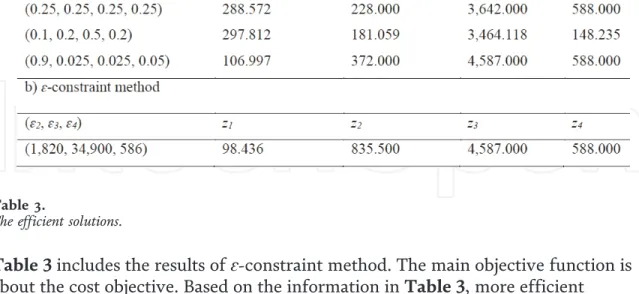
In this research, the General Algebraic Modeling System (GAMS) software is employed to write the codes and find the solutions. First, different weights are devoted to the objective functions and the problem is solved. Each solution of the multi-objective model is called efficient solution. Efficient solutions cannot be improved without scarifying other objective functions [46, 51–56]. The results have been collected inTable 3. As it can be seen, the weights are assigned between 0 and 1. The efficient solutions are presented to the decision-makers. The second part of
Table 2.
Recommended number and amount of food guided servings in a month for 51+ year-old females.
Table 3includes the results ofɛ-constraint method. The main objective function is about the cost objective. Based on the information inTable 3, more efficient
solutions have been obtained in weighted-sums method. Consequently, this method is selected to solve the mathematical model.
One of the efficient solutions inTable 3 has been obtained by considering equal weights (w1= 0.25,w2= 0.25,w3= 0.25, andw4 = 0.25). The values of the decision variables related to this solution are as follows:N1.3.1= 11.250, N1.3.2= 11.250, N2.2.1= 4.667,N2.2.2= 4.667,N3.4.1= 3.775,N3.4.2= 3.775,N4.1.1= 7.500, and
N4.1.2= 7.500. In other words, Food 1 in Group 3 in Periods 1 and 2, Food 2 in Group 2 in Periods 1 and 2, Food 3 in Group 4 in Periods 1 and 2, and Food 4 in Group 1 in Periods 1 and 2 should be purchased to have optimal solution.
7. The optimization model under uncertainty
In reality, several parameters are uncertain. In this section, the effects of uncer- tainty in two parameters including cost of foods and amount of food guide servings per month are examined in the mathematical model. These two parameters are very important factors of food items. Suppose thaturepresents a scenario amongU scenarios. The decision variables (nonnegative variables in this case) are written based on each scenario [39].Aihtuis defined as cost of foodiin food grouphand periodtin scenariou. It is noticeable that the costs of foods in different stores are usually different. Furthermore,Ψhturepresents the amount of food guide servings per month in food grouphin periodtin Scenariou. muis introduced as the probability related to Scenariou.The new optimization model under uncertainty is written as follows:
Min z1¼X
u
X
t
X
h
X
i
muAihtuNihtu (20) Min z2 ¼X
u
X
t
X
h
X
i
muaihKihNihtu (21) Min z3 ¼X
u
X
t
X
h
X
i
muaihLihNihtu (22) Max z4 ¼X
u
X
t
X
h
X
i
muaihMihNihtu (23)
Table 3.
The efficient solutions.