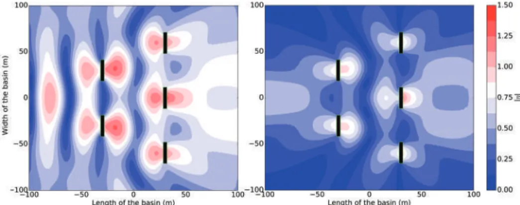
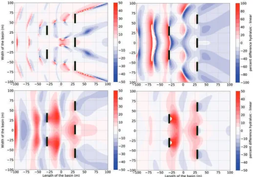
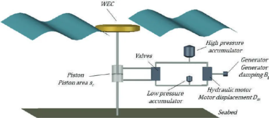
Renewable Energy in Marine Environment

For certain types of WECs, namely heaving cylindrical WECs, the PTO system strongly modifies the motion of the WECs. The impact of the hydraulic PTO system on the output power and 'near-field' surface heights of the 5-WEC array is compared to the base case of a linear PTO system.

PTO Model Development 1. Equations of Motion

The PTO force applied by the hydraulic PTO system always has the opposite sign to the speed of the swaying cylindrical WEC. The calculation of the pressure in the low pressure accumulator, pl(tj), is done in the same way.

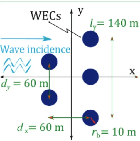
Figure 1. Schematic representation hydraulic PTO for heaving cylindrical WEC.

Modelled WECs and Input Wave Conditions

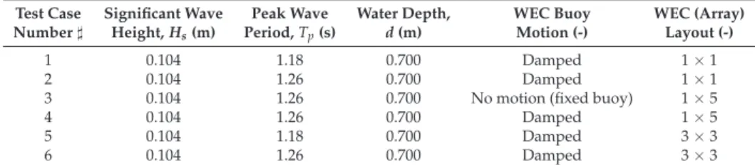
The optimal hydraulic PTO system damping coefficients for the heaving cylindrical WEC for the studied wave conditions are summarized in Table 3. The hydraulic PTO system used on the OSWEC exerts a torque,TPTO(t) = fPTO(t)·(t), depending on the PTO forcefPTO and the lever.

Table 2. Optimal linear B PTO coefﬁcients for a heaving cylindrical WEC (10 6 × kg/s) and OSWEC (10 6 × (kg · m 2 )/s).

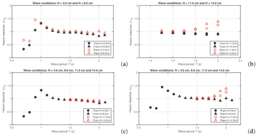
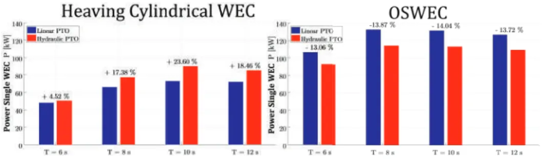
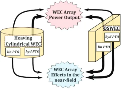
Comparing the Effects of a Linear to a Hydraulic PTO System for a Single Heaving Cylindrical WEC and a Single OSWEC

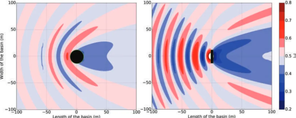
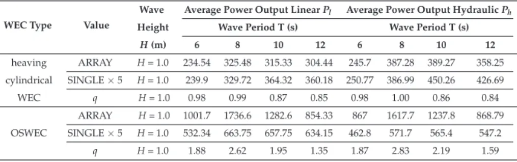
It can be seen that there is a noticeable increase in the average power output for the PTO hydraulic system (Ph) compared to the linear one (Pl) for the case of the rising cylindrical WEC for periods T≥8.0 s. We calculate the wave field around a single WEC for each of the incident wave conditions presented in Table 1.

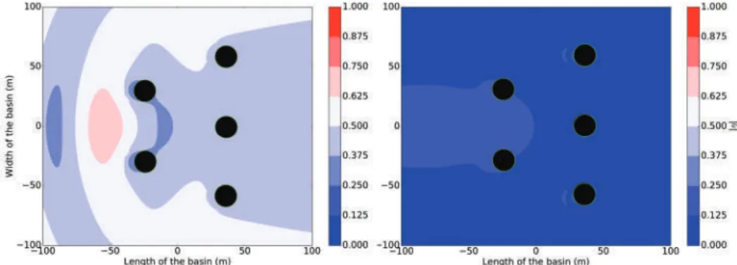
Figure 6. Bar chart showing the power output for one WEC with linear PTO system (P l ) (purple) and hydraulic PTO system (P h ) (red) with the percentage difference between the two

Analyzing the Power Production and the Near-Field Effects for an Array of 5 WECs With a Hydraulic PTO System

We can observe this in a contour plot of the total and the perturbed wavefield for T= 10.0 s for the heaving cylindrical WEC array with a linear PTO system in Figure 16. We start by looking at the effect of the hydraulic PTO system for the case of the heaving cylindrical WEC.

Figure 10. Plan view of the array layout for ﬁve heaving cylindrical WECs. The incident wave propagates from the left.

Discussion

Furthermore, the effect of the change in the PTO system of the pitching cylindrical WEC is not necessarily reflected in the output power of the pitching cylindrical WEC array. In contrast to the heaving cylindrical WEC case, we also note that a change in the PTO system reduces the ηin le of the WEC array, increasing the areas of destructive interference.

Figure 23. Schematic diagram showing the relationship between the PTO system impacts of the two types of WECs in an array

Conclusions

In Proceedings of the 10th European Conference on Wave and Tidal Energy, Aalborg, DK, USA, 2–5 September 2013. In Proceedings of the Twelfth European Conference on Wave and Tidal Energy, Cork, Ireland, 27 August–1. September 2017; p.

Irregular Wave Validation of a Coupling

Introduction
Generic Coupling Methodology
Application of the Coupling Methodology between the Wave Propagation Model, MILDwave, and the Wave–Structure Interaction Solver NEMOH for Irregular Waves
Validation Strategy of the Coupling Methodology between the Wave Propagation Model, MILDwave, and the Wave–Structure Interaction Solver, NEMOH
Validation Results
Discussion
Conclusions

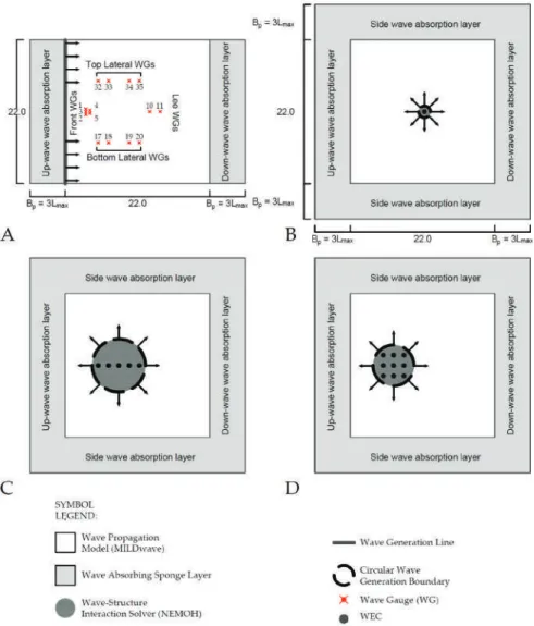
Section 3 illustrates the MILDwave-NEMOH coupled model, including a detailed description of the coupling methodology implementation, the wave propagation solver MILDwave, and the wave structure interaction solver NEMOH. Finally (Step 4), the total wavefield due to the presence of the structure(s) is obtained as the superposition of the incident wavefield and the disturbed wavefield in the wave propagation model.

Figure 1. Set-up of the different numerical wave basins used in MILDwave. The wave gauges (WGs) are represented by the x symbol and numbered as they appear in the WECwakes experimental data-set.

On the Variation of Turbulence in a High-Velocity Tidal Channel

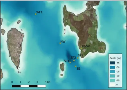
Data Collection and Methodology 1. Sensor Deployment

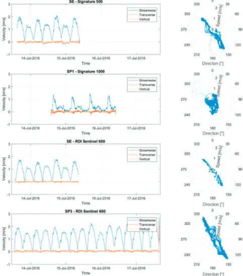
In addition, the X-band land-based radar system was used to remotely measure wave conditions and surface current; further details on the measurement of flow characteristics using radar can be found in [27]. This study uses an approach where the velocities from the four beams are used to calculate the flow vector in a number of coordinate systems [28,29]. Uv white velocities are calculated based on the same 600 s window where the mean flow direction is subtracted from the outflow direction.

Figure 1. Sensor deployment locations for the Fall of Warness measurement campaign with the bathymetry provided by UK Hydrographic Ofﬁce.

Data Analysis and Results 1. Flow Characteristics

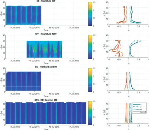
The velocity profiles shown provide further detail of the flow characteristics around the Warness Drop. The two left columns show the average flood tide (blue) and the two right columns show the average ebb tide results (red), where the individual profiles for the three maximum flood and ebb velocities are shown in grey. However, the shear stresses are much greater for the upper part of the water column.

Figure 3. Left: Average ﬂow velocity vectors over 10 min in the streamwise coordinate system for the SE—Signature 500, SP1—Signature 1000, SE—Sentinel V50 and the SP3—Workhorse

Discussion

This sensor experiences a highly disturbed tidal flow pattern, with flow rates decreasing significantly during low tide and a later part of high tide. This shows the spatial variability of the flow field, where large differences in flow and turbulence characteristics occur over a short distance. The SP3 sensor experiences significant turbulence and flow disturbances, making it a poor location for turbine placement.

Conclusions

However, during turbulence analysis, this apparent smoothing of the velocity variation causes significant effects on the turbulence parameters. All results from the spatially distributed sensors show turbulence levels consistent with previous literature with similar flow rates for tidal energy test sites where turbulence intensities are on the order of 0.1 for the height of the center water depth. The writing of the manuscript was led by C.G., with contributions to individual sections and editorial support by A.V.

Implementation of Open Boundaries within a

Two-Way Coupled SPH Model to Simulate Nonlinear Wave–Structure Interactions

Smoothed Particle Hydrodynamics

The contribution of the neighboring particles is weighted, based on their distance to particles, using a kernel function W, and a smoothing length tehSPH. If ΔVb=mb/ρb, with a band that determines the mass and density of particle b, then Equation (2):. 3) The choice of the kernel function has a great influence on the performance of the SPH method. Physically, the delta-SPH formulation can be defined as adding the Laplacian of the density field ∇2ρ to the continuity equation.

Boundary Conditions in DualSPHysics 1. Open Boundary Conditions

This is necessary to have full kernel support for fluid particles near the threshold boundary. As illustrated in Figure 1, the positions of the phantom nodes are calculated by mapping the locations of the buffer particles in the fluid domain, along a direction that is perpendicular to the open boundary. Second, there are no phantom nodes to extrapolate physical quantities from the fluid domain to the buffer particles.

Figure 1. Sketch of the implemented open boundary model, adapted from Tafuni et al. [24].

Coupling Methodology Using DualSPHysics and OceanWave3D

At the end of the time step, DualSPHyics returns the measured surface height near the inlet and outlet. The WEC is located at a distance of 1.52 m from the inlet boundary of the numerical domain. (c) the horizontal thrust acting on the WEC and (d) the heaving motion of the WEC.

Figure 3. Sensitivity analysis on the number of buffer particle layers n l necessary for accurate wave propagation, represented by the ratio K D along the ﬂuid domain.

Accurate and Fast Generation of Irregular Short Crested Waves by Using Periodic Boundaries in a

Numerical Methodology

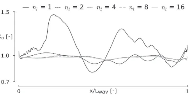
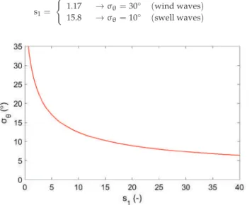
In this method, the wave propagation angles are randomly selected according to the cumulative distribution function of the directional distribution function, D(f,θ), and are assigned to each frequency component. Several semi-empirical proposed formulations of the directional distribution function, D(f,θ), have been reported, most of which consider the distribution function to be independent of the wave frequency. In the present study, a single wave generation line parallel to the y-axis is combined with periodic lateral boundaries at the top and bottom of the domain.

Figure 2. Relation between the directional spreading parameter, s 1 , and the spreading standard deviation, σ θ .

Results by the Model, MILDwave

Figure 5 shows the plan views of the resulting disturbance coeﬃcient, kd, and water surface elevation, η, in the inner computational domain at time t=80 T, where T is the wave period, for each wave generation layout for a wave propagation angle of θ= 30◦. In Figure 6, the mean (Emean) and maximum (Emax) value of the calculated absolute errors for each wave generation layout for a variety of wave propagation angles are plotted. In addition, the comparison between the L-shaped wave generation layout and the arc-shaped wave generation layout reveals that in the case of the latter, the wave diffraction is avoided due to the intersection of the two generation lines [10].

Figure 4. Deﬁnition sketch of three wave generation layouts: (a) L-shaped, (b) arc-shaped, (c) line-shaped with periodic lateral boundaries

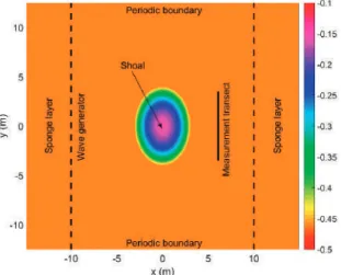
Numerical Validation Using the Vincent and Briggs Shoal Experiment

MILDwave with the addition of the periodic boundaries correctly predicts the wave focusing behind the school for the case of irregular long crested waves where the wave height is strongly influenced by the change of the water depth. The results indicate that the MILDwave model with the addition of the periodic boundaries is able to reproduce a homogeneous wavefield (especially when the Sand and Mynett method is used) as well as the target frequency spectrum and the target direction spectrum. Assessment of the power output of a two-array clustered WEC farm using a BEM solver coupling and a wave propagation model.Energy.

Figure 12. Bottom levels of the experimental setup used by Vincent and Briggs, as it is implemented in the numerical domain in MILDwave.

Large-Scale Experiments to Improve Monopile Scour Protection Design Adapted to Climate Change—The

Stability of Scour Protection Around Monopiles: Governing Physics 1. Governing Physics at A Glance

In the presence of a monopile, flows are accelerated in the direction surrounding the monopile, due to the contraction of the streamlines. Amplification of shear stresses increases the erosive potential of the flow. In the case of a monopile protected by a scratch protection, the scratch protection material can be removed, eventually leading to failure of the scratch protection.

Experimental Setup 1. Experimental Facility

Each model is attached to a mounting base that is attached to the bottom of the sandbox (Figure 3a). The location of the sand pit (details shown in Figure 3a,c) in relation to the wave generator is shown in Figure 1. The filling of the sand pit was carried out after the installation of each of the monopile scale models (Figure 3c).

Figure 1. Sketch of the fast ﬂow facility (FFF) ﬂume channels including the position of the scale models.

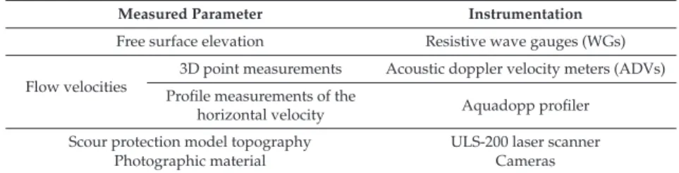
Instrumentation Setup

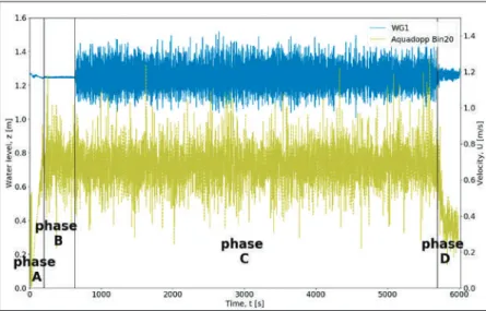
During the calibration stage, the Aquadopp is positioned at x=30.0 m and y=0.0 m in the main current channel, on the planned position of the monopile. The topography of the scour protection model is measured using a ULS-200 underwater laser scanner operating at 7 Hz (7 mm/s) mounted in a traverse system above the scour protection model (Figure8). After each wave train, the topography of the abrasion protection model is measured using the laser scanner.

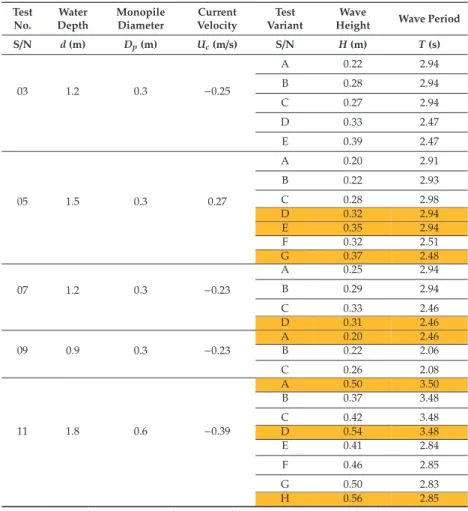
Table 1. Measured parameters and instrumentation.

Experimental Test Program

The start of movement tests with clear movement of the anti-scratch material is highlighted. Such a scratch protection design allows very little movement of the scratch protection material. The intrinsic properties of the anti-scratch material, i.e., the average stone diameter, D50, and the material composition gradation, D85/D15, are shown in Table 6.

Table 4. Onset of motion measured test conditions. The highlighted conditions are the ones where the motion of scour protection material is spotted

Results and Discussion

The initial state of the scour protection model can be seen in the left panel (Figure 17a), and the final state after 3000 waves in the right panel (Figure 17b). From figures 17 and 18 it is clear that the scour protection material has undergone damage caused by the hydrodynamic effect of the flow. Based on the tested hydrodynamic conditions, the measured damage and the predicted damage of the scour protection material are presented in Table 10.

Figure 12. Test 04_B measurement of WG1 (left vertical axis) and Aquadopp at bin 20 (right vertical axis) with test phases: (“phase A”) Initialization of the test (time: 0–200 s); (“phase B”) Current stabilization (time: 200–633 s); (“phase C”) Wave Genera

Moored Cubic Box

Experimental Setup 1. Description of the Models

The front open side of the OWC WEC model faces the incoming waves. The center of gravity of the OWC WEC model is located on the symmetry plane of the WEC. The center of gravity of the OWC WEC or box model is located at the origin of this global coordinate system.

Figure 1. Geometry of ﬂoating models: (a) BOX; (b) OWC WEC.

BOX model Experimental Results

For the wave generation system, the uncertainties are related to the measurement of wave surface height and wave period. The results are discussed in terms of the modification of the wave field due to the presence of the BOX model. The heave (Figure 5c) and pitch (Figure 5d) movements of the BOX model are regular and the amplitude of the movement is stable.

OWC WEC Model Experimental Results 1. OWC WEC Motion Response

This section discusses the sensitivity of the mooring line tensions to the unbalanced mooring line lengths. The study focuses on the comparison of the OWC WEC movement and of the water surface height in the chamber. First, by applying a series of nonlinear regular wave conditions, the motion response of the OWC WEC model is recorded.