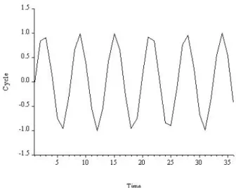
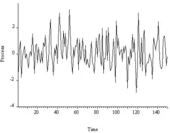
4It is called white noise, by analogy with white light, which is composed of all the colors of the spectrum, in equal amounts. We read 'y is independently and identically distributed as normal, with zero mean and constant variance', or simply 'y is Gaussian white noise'. In Figure 6.6 we show an example path of Gaussian white noise, with length T = 150, simulated on a computer. 6Another name for independent white noise is strong white noise, as opposed to standard serially uncorrelated weak white noise.
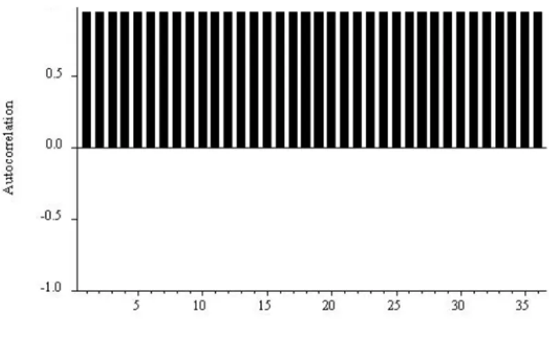
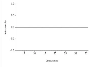
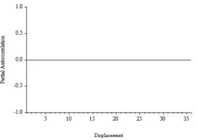
Remember that the disturbance in a regression model is typically assumed to be white noise of some kind. For a white noise process, all partial autocorrelations beyond displacement 0 are zero, which again follows from the fact that white noise is, by construction, serially uncorrelated. Second, the goal of all time series modeling (and 1-step-ahead forecasting) is to reduce the data (or 1-step-ahead forecast errors) to white noise.
So far, we have characterized white noise in terms of its mean, variance, autocorrelation function, and partial autocorrelation function. Conditional and unconditional means and variances are the same for an independent series of white noise; there is no dynamism in the process and thus no dynamism in conditional moments.
Estimation and Inference for the Mean, Autocor- relation and Partial Autocorrelation Functions
A key result, which we simply assert, is that if a series is white noise, then the distribution of the sample autocorrelations in large samples is . The sample autocorrelations of a white noise series are approximately normally distributed, and the normal is always a convenient distribution to work with. Finally, the variance of the sample autocorrelations is approximately 1/T (equivalently, the standard deviation is 1/√ . T ), which is easy to construct and remember.
Thus, if the sequence is white noise, approximately 95% of the sample autocorrelations should fall within the interval 0± 2/√. That is, if the series consists of white noise, approximately 95% of the sample's partial autocorrelations should fall in the interval ±2/√. A “correlogram analysis” simply means examination of the sample's autocorrelation and partial autocorrelation functions (with two standard error bands), along with related diagnostics, such as Q statistics.
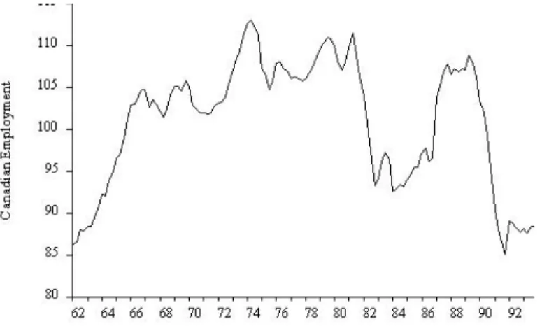
Canadian Employment I: Characterizing Cycles
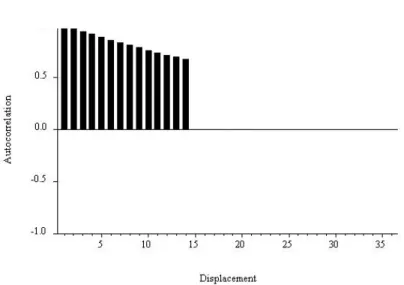
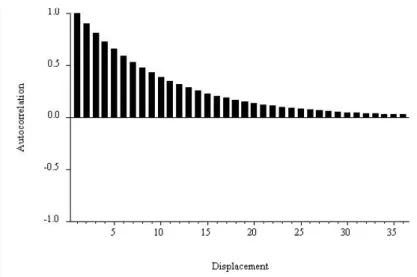
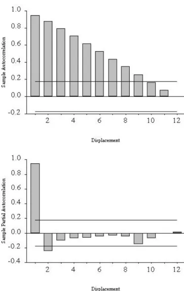
Moreover, the autocorrelation and partial autocorrelation functions of the sample have special forms: the autocorrelation function shows a slow one-sided damping, while the partial autocorrelation function stops at displacement 2. 15 We do not show the autocorrelation or partial autocorrelation of the sample at displacement 0, because they , as we mentioned earlier, are equivalent in construction to 1.0 and therefore do not convey any useful information. That's because at displacement 1 there are no prior lags to take into account when calculating the sample's partial autocorrelation, so it is equal to the sample's autocorrelation.
Modeling Cycles With Autoregressions
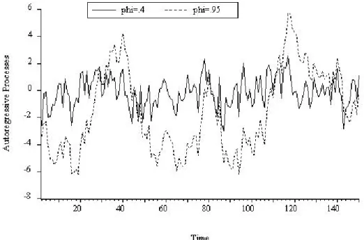
We begin by characterizing the autocorrelation function and related quantities under the assumption that the AR model is the DGP.17 These characterizations have nothing to do with data or estimates, but are crucial for developing a basic understanding of the properties of the models , That. They allow us to make statements like: “If the data were truly generated by an autoregressive process, then we would expect its autocorrelation function to have the property x.” Armed with that knowledge, we use the autocorrelations and partial autocorrelations from the sample , in combination with the AIC and the SIC, to propose candidate models, which we then estimate. The fluctuations in the AR(1) with parameterφ = .95 seem much more persistent than those of the AR(1) with parameter φ = .4.
The condition is that all roots of the autoregressive lag operator polynomial must be outside the unit circle. Ultimately, the ε's are the only thing that moves y, so it stands to reason that we should be able to express y in terms of ε's history. And we know γ(0); it is merely the variance of the process, which we have already shown to be.
For displacement 1, the partial autocorrelations are simply the parameters of the process (.4 and .95, respectively), and for longer displacements the partial autocorrelations are zero. In our discussion of the AR(p) process, we forego mathematical derivations and rely instead on parallels with the AR(1) case to establish intuitions for its key properties. The autocorrelation function for the general AR(p) process, like that of the AR(1) process, decays gradually with displacement.
Finally, the partial autocorrelation function AR(p) has a sharp discontinuity at shift p, for the same reason that the partial autocorrelation function AR(1) has a sharp discontinuity at shift 1. The key insight is that, despite from the fact that its qualitative behavior (gradual smoothing) matches that of the AR(1) autocorrelation function, however it can exhibit a richer variety of patterns, depending on the order and process parameters. For example, it can have damped monotonic decay, as in the AR(1) case with a positive coefficient, but it can also have damped oscillations in ways that AR(1) cannot.
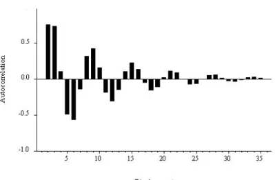
In the AR(1) case, the only possible oscillation occurs when the coefficient is negative, in which case. This occurs when some roots of the autoregressive lag operator are polynomially complex.20 Consider, for example, the AR(2) process,. Because the roots are complex, the autocorrelation function oscillates, and because the roots are close to the unit circle, the oscillation damps slowly.
Canadian Employment II: Modeling Cycles
Forecasting Cycles with Autoregressions
Based on that information set, we want to find the optimal forecast of y at some future time T + h. The optimal forecast is the one with the smallest loss on average, that is, the forecast that minimizes the expected loss. It turns out that in rather weak conditions the optimal forecast is the conditional average.
In general, the conditional mean need not be a linear function of the elements of the information set. Because linear functions are particularly tractable, we prefer to work with linear forecasts – forecasts that are linear in the elements of the information set – by finding the best linear approximation to the conditional mean, called the linear projection. This explains the common term "linear least squares prediction." The linear projection is often very useful and accurate because the conditional mean is often close to linear.
For autoregressions, a very simple recursive method is available for computing optimal h step-by-point predictions, for any desired h. First, we construct the optimal one-step-ahead prediction, and then we construct the two-step-ahead optimal prediction, which depends on the one-step-ahead optimal prediction we have already constructed. Then we construct the optimal three-steps-ahead prediction, which depends on the already calculated two-steps-ahead prediction, which we have already made, and so on.
Then, projecting the right-hand side onto the time-T information set, we get yT+1,T = φyT. Hence the name "chain rule of prediction". Note that, for the AR(1) process, only the most recent value of y is needed to construct optimal forecasts, for each horizon, and for the general AR(p) process only the most recent p values of y are needed. It is worth noting that thanks to Wold's chain rule we have now solved the FRV problem for autoregressions, as we did previously for cross sections, trends and seasons.
Using Wold's chain rule, we have already derived the formula for yT+h,T, so all we need is the h-step-ahead prediction error variance, σh2.
Canadian Employment III: Forecasting
As usual, in reality the parameters are unknown and thus must be estimated, so we turn infeasible predictions into feasible (“operational”) predictions by introducing the usual estimates where unknown parameters appear. In addition, and also as usual, we can account for non-normality and parameter estimation uncertainty using simulation methods. In normality, we still need the corresponding prediction-error variances of the step h, we infer from the moving average representation.
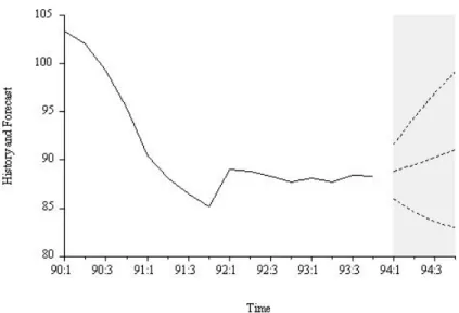
In Figure 6.21 we show the employment history, the 4-quarter-ahead AR(2) extrapolation forecast and the realization. Eventually the unconditional mean is approached, and eventually the error bands become flat, but only for very long horizon forecasts, due to the high employment persistence captured by the AR(2) model.
Exercises, Problems and Complements
A telltale sign of the slowly evolving nonstationarity associated with trend is a sample autocorrelation function that damps extremely slowly. Fit appropriate trend models, obtain the model residuals, calculate their sample autocorrelation functions, and report your results. An indicative sign of seasonality is a sample autocorrelation function with sharp peaks at the seasonal displacements etc. for quarterly data etc. for monthly data, and so on).
Recall the Durbin-Watson test statistic discussed in Chapter 2. so the Durbin-Watson test is effectively only based on the first autocorrelation of the sample and is actually just testing whether the first autocorrelation is zero. Furthermore, the Durbin-Watson test is not valid in the presence of lagged dependent variables.21. Therefore, for example, we do not report (and the software does not actually calculate) the p-value for the Q statistic associated with the residual correlogram of our recruitment prediction model until m > K. b) Durbin's h test is an alternative to the Durbin-Watson test. 21 In accordance with standard, if not entirely appropriate, practice, the Durbin-Watson statistic is frequently reported and examined throughout this book, even when lagged dependent variables are included.
We always supplement the Durbin-Watson statistic, however, with other diagnostics such as the residual correlogram, which remains valid in the presence of lagged dependent variables and which almost always produces the same conclusion as the Durbin-Watson statistic. with the Durbin-Watson test, is designed to detect first-order serial correlation, but is valid in the presence of lagged dependent variables. Make your expressions functional for both forecasts and forecast error variances by entering least squares estimates where unknown parameters appear and use them to produce an operation. As we have seen, calculating the variances of the prediction errors that accept the uncertainty of the parameter estimates is very difficult; this is one reason why we have ignored it.
In covariance stationary environments, the forecast error variance approaches the (finite) unconditional variance as the horizon grows. We usually expect the variance of the forecast error to increase monotonically with the horizon, but this is not necessary. Even in covariance stationary environments, the forecast error variance need not converge to the unconditional variance as the forecast horizon lengthens; instead, it can grow indefinitely.
With known parameters, the point forecast will converge to the trend as the horizon increases, and the forecast error variance will converge to the unconditional variance of the AR(1) process.
Notes