Data classification using genetic programming.

(1)

Data Classification using Genetic Programming

by

Emmanuel Dufourq

Submitted in fulfilment of the academic requirements for the degree of

Master of Science in the

School of Mathematics, Statistics, and Computer Science, University of KwaZulu-Natal,

Pietermaritzburg

February 2015 As the candidate’s supervisor I have/have not approved this thesis/dissertation for submission.

Name: Professor Nelishia Pillay

Signature

Date

(2)

i

PREFACE

The experimental work described in this dissertation was carried out in the School of Mathematics, Statistics, and Computer Science, University of KwaZulu-Natal, Pietermartizburg, from February 2013 to February 2015, under the supervision of Professor Nelishia Pillay.

These studies represent original work by the author and have not otherwise been submitted in any form for any degree or diploma to any tertiary institution. Where use has been made of the work of others it is duly acknowledged in the text.

Supervisor: Professor Nelishia Pillay

Signature

Candidate: Emmanuel Dufourq

Signature

(3)

DECLARATION 1 - PLAGIARISM

I, Emmanuel Dufourq (student number: 208517550) declare that

1. The research reported in this thesis, except where otherwise indicated, is my original research.

2. This thesis has not been submitted for any degree or examination at any other university.

3. This thesis does not contain other persons’ data, pictures, graphs or other information, unless specifically acknowledged as being sourced from other persons.

4. This thesis does not contain other persons’ writing, unless specifically acknowledged as being sourced from other researchers. Where other written sources have been quoted, then: a. Their words have been re-written but the gen- eral information attributed to them has been referenced b. Where their exact words have been used, then their writing has been placed in italics and inside quotation marks, and referenced.

5. This thesis does not contain text, graphics or tables copied and pasted from the Internet, unless specifically acknowledged, and the source being detailed in the thesis and in the References sections.

Signature

(4)

iii

DECLARATION 2 - PUBLICATIONS

DETAILS OF CONTRIBUTION TO PUBLICATIONS that form part and/or include research presented in this thesis

• Publication 1: E. Dufourq and N. Pillay, ”Incorporating Adaptive Discretiza- tion into Genetic Programming for Data Classification,” in proceedings of the 2013 World Congress on Information and Communication Technologies (WICT 2013), pp. 127-133, 2013

• Publication 2: E. Dufourq and N. Pillay, ”A Comparison of Genetic Pro- gramming Representations for Binary Data Classification,” in proceedings of the 2013 World Congress on Information and Communication Technologies (WICT 2013), pp. 134-140, 2013

• Publication 3: E. Dufourq and N. Pillay, ”A Preliminary Study on the Reuse of Subtrees Within Decision Trees in a Genetic Programming Context for Data Classification,”in proceedings of the 2013 World Congress on Information and Communication Technologies (WICT 2013), pp. 287-292, 2013

• Publication 4: E. Dufourq and N. Pillay, ”Hybridizing Evolutionary Algo- rithms for Creating Classifier Ensembles,” in proceedings of the 2014 Sixth World Congress on Nature and Biologically Inspired Computing (NaBIC 2014), pp. 84-90, 2014

Supervisor: Professor Nelishia Pillay

Signature

(5)

Abstract

Genetic programming (GP), a field of artificial intelligence, is an evolutionary algorithm which evolves a population of trees which represent programs. These programs are used to solve problems. This dissertation investigates the use of genetic programming for data classification. In machine learning, data classification is the process of allocating a class label to an instance of data. A classifier is created in order to perform these allocations. Several studies have investigated the use of GP to solve data classification problems. These studies have shown that GP is able to create classifiers with high classification accuracies. However, there are certain aspects which have not previously been investigated.

Five areas were investigated in this dissertation. The first was an investigation into how discretisation could be incorporated into a GP algorithm. An adaptive discretisation algorithm was proposed, and outperformed certain existing methods.

The second was a comparison of GP representations for binary data classification.

The findings indicated that from the representations examined (arithmetic trees, decision trees, and logical trees), the decision trees performed the best. The third was to investigate the use of the encapsulation genetic operator and its effect on data classification. The findings revealed that an improvement in both training and test results was achieved when encapsulation was incorporated. The fourth was an investigative analysis of several hybridisations of a GP algorithm with a genetic algorithm in order to evolve a population of ensembles. Four methods were proposed and these methods outperformed certain existing GP and ensemble methods. Finally, the fifth area was to investigate an ensemble construction method for classification.

In this approach GP evolved a single ensemble. The proposed method resulted in an improvement in training and test accuracy when compared to the standard GP algorithm.

The methods proposed in this dissertation were tested on publicly available data sets, and the results were statistically tested in order to determine the effectiveness of the proposed approaches.

(6)

v

Acknowledgements

The financial assistance of the National Research Foundation (NRF) towards this research is hereby acknowledged. Opinions expressed and conclusions arrived at, are those of the author and are not necessarily to be attributed to the NRF.

I would like to thank the Centre for High Performance Computing for granting access to their resources.

I would also like to thank my supervisor, Professor Nelishia Pillay, for her guid- ance, as well as my family and friends who have encouraged and supported me, especially my parents. I would like to thank the technical staff from the School of Mathematics, Statistics and Computer Science for their support and for enabling me to perform my simulations.

(7)

Contents

PREFACE i

DECLARATION 1 - PLAGIARISM ii

DECLARATION 2 - PUBLICATIONS iii

Abstract iv

Acknowledgements v

Contents vi

List of Figures xii

List of Tables xv

List of Algorithms xx

1 Introduction 1

1.1 Purpose of the Study . . . 1

1.2 Objectives . . . 1

1.3 Contributions . . . 3

1.4 Dissertation Layout . . . 4

2 Genetic Programming 6 2.1 Introduction . . . 6

2.2 Introduction to Genetic Programming . . . 6

2.3 Overview of the Generational GP Algorithm . . . 7

2.4 Terminal Set . . . 8

2.5 Function Set . . . 9

2.6 Tree Based GP . . . 9 vi

(8)

CONTENTS vii

2.7 Initial Population Generation . . . 10

2.7.1 Full method . . . 11

2.7.2 Grow method . . . 12

2.7.3 Ramped half and half . . . 12

2.8 Fitness . . . 14

2.8.1 Fitness cases . . . 14

2.8.2 Fitness functions . . . 15

2.9 Selection Methods . . . 16

2.9.1 Fitness proportionate selection . . . 17

2.9.2 Tournament selection . . . 18

2.10 Genetic Operators . . . 19

2.10.1 Reproduction . . . 20

2.10.2 Mutation . . . 20

2.10.3 Crossover . . . 20

2.11 Termination . . . 21

2.12 Strongly-Typed GP . . . 22

2.13 GP Control Models . . . 22

2.14 Modularisation . . . 23

2.14.1 Encapsulation . . . 24

2.14.2 Compression . . . 25

2.15 GP and Bloat . . . 26

2.16 Strengths and Weaknesses of GP . . . 26

2.16.1 Strengths . . . 26

2.16.2 Weaknesses . . . 26

2.17 Conclusion . . . 27

3 Data Classification 29 3.1 Introduction . . . 29

3.2 Introduction to Data Classification . . . 29

3.3 Definitions . . . 30

3.3.1 Instance . . . 30

3.3.2 Attribute . . . 31

3.3.3 Class . . . 32

3.3.4 Data set . . . 32

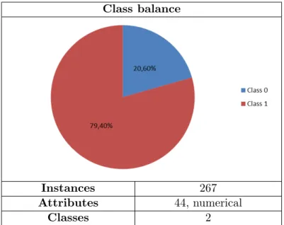
3.3.5 Class balance . . . 33

3.3.6 Classifier . . . 33

3.4 Performance Measures . . . 34

3.4.1 Confusion matrix . . . 34

3.4.2 Sensitivity and specificity . . . 35

(9)

3.4.3 Receiver operating characteristics . . . 36

3.5 Evaluating Classifiers . . . 37

3.5.1 Train/test split . . . 38

3.5.2 K-fold cross-validation . . . 38

3.5.3 Leave-one-out . . . 39

3.5.4 Bootstrapping . . . 39

3.6 Previous Work on Data Classification . . . 40

3.6.1 K-nearest neighbour . . . 40

3.6.2 Decision trees . . . 41

3.6.3 Artificial neural networks . . . 43

3.6.4 Na¨ıve bayes . . . 43

3.6.5 Evolutionary algorithms . . . 44

3.7 Active Research Areas in Data Classification . . . 46

3.7.1 Feature selection . . . 46

3.7.2 Missing values . . . 47

3.7.2.1 Discarding missing values . . . 48

3.7.2.2 Imputation . . . 48

3.7.2.3 Missing values and decision trees . . . 48

3.7.3 Ensemble classifiers . . . 49

3.7.4 Discretisation . . . 51

3.8 Software . . . 53

4 GP and Data Classification 56 4.1 Introduction . . . 56

4.2 GP and Decision Trees . . . 56

4.2.1 Advantages and disadvantages of GP decision trees . . . 60

4.2.2 Summary of the findings . . . 61

4.3 GP and Arithmetic Trees . . . 62

4.3.1 Binary classification . . . 62

4.3.2 Multiclass classification . . . 68

4.3.3 Advantages and disadvantages of GP arithmetic trees . . . . 74

4.4 GP and Logical Trees . . . 77

4.4.1 Advantages and disadvantages of GP logical trees . . . 80

4.5 GP and Other Representations . . . 81

4.6 GP and Ensemble Classifiers . . . 83

4.6.1 Strengths and weaknesses of GP ensembles . . . 88

(10)

CONTENTS ix

4.7 Strengths and Weaknesses of Applying GP to Data Classification . 89 4.7.1 Strengths . . . 89

4.7.2 Weaknesses . . . 90

4.8.1 GP for data classification . . . 91

4.8.2 GP representations for data classification . . . 92

4.8.3 GP discretisation for data classification . . . 94

4.8.4 GP encapsulation for data classification . . . 94

4.8.5 GP ensembles for data classification . . . 94

5 Methodology 96 5.1 Introduction . . . 96

5.2 Addressing the objectives . . . 96

5.3 Statistical testing . . . 98

5.4 Data Sets . . . 99

5.4.1 Characteristics of data sets for data classification problems . 99 5.4.2 Binary data sets . . . 100

5.4.3 Multiclass data sets . . . 106

5.4.4 Rationale behind the selected data sets . . . 111

5.5 GP System . . . 113

5.6 Performance Measures . . . 114

5.7 Technical Specifications . . . 114

6 Adaptive Discretisation for GP 116 6.1 Introduction . . . 116

6.2 Proposed Discretisation Methods for GP . . . 116

6.2.1 Equal Width Intervals (EWI) . . . 118

6.2.2 GP Evolved Intervals (GPEI) . . . 119

6.3 Experimental Setup . . . 123

6.3.1 Data sets . . . 124

6.3.2 GP parameters . . . 125

7 GP Representations for Binary Classification 126 7.1 Introduction . . . 126

7.2 GP Representations for Binary Classification . . . 126

7.2.1 Arithmetic trees . . . 126

7.2.2 Decision trees . . . 127

(11)

7.2.3 Logical trees . . . 128

7.3.1 Data sets . . . 131

8 GP Encapsulation for Data Classification 133 8.1 Introduction . . . 133

8.2 Incorporating Encapsulation into GP for Data Classification . . . . 133

8.2.1 Decision trees and encapsulation . . . 133

8.2.2 Maintaining the most called subtrees . . . 136

8.3.1 Data sets . . . 139

9 Hybridising Evolutionary Algorithms 141 9.1 Introduction . . . 141

9.2 Proposed Hybridisation of GP and GA . . . 141

9.2.1 GA encoding . . . 143

9.2.2 GA run after the last GP generation (GA-at-end) . . . 144

9.2.3 GA run after each GP generation (GA-after-each-gen) . . . . 145

9.2.4 GA with hill climbing (GA-with-HC) . . . 146

9.2.5 Steady state GA (SSGA-GP) . . . 146

9.3.1 Data sets . . . 150

9.3.2 GP and GA parameters . . . 150

10 GP Ensemble Construction 152 10.1 Introduction . . . 152

10.2 Proposed Ensemble Construction . . . 152

10.2.1 Selecting a tree to add to the ensemble . . . 153

10.2.2 Ensemble evaluation . . . 154

10.2.3 Evaluating the GP trees using weights . . . 155

10.2.4 Updating the weights . . . 158

10.3.2 Data sets . . . 161

(12)

CONTENTS xi

11 Results and Discussion 163

11.1 Introduction . . . 163

11.2 GP Discretisation . . . 163

11.3 GP Representations for Binary Classification . . . 168

11.4 GP Encapsulation . . . 173

11.5 Hybridisation of GA and GP . . . 176

11.6 GP Ensemble Construction . . . 185

12 Conclusions and Future Work 192 12.1 Objective 1 - GP Discretisation . . . 192

12.2 Objective 2 - GP Representations for Binary Classification . . . 193

12.3 Objective 3 - GP Encapsulation . . . 194

12.4 Objective 4 - Hybridising GA and GP . . . 194

12.5 Objective 5 - GP Ensemble Construction . . . 195

Bibliography 197 Appendices 212 A User Manual 213 A.1 Program Requirements . . . 213

A.2 Starting the Program . . . 214

A.3 Selecting an Experiment to Run . . . 214

A.4 Starting an Experiment . . . 215

A.4.1 Selecting a data set . . . 215

A.4.2 Executing the experiment . . . 216

(13)

List of Figures

2.1 Illustrating nodes with different arity. . . 9

2.2 GP tree. . . 10

2.3 Illustrating the depth of each node within a tree. . . 11

2.4 A tree created using the full method (left), and a tree created using the grow method (right). . . 12

2.5 Illustrating an initial population created using the ramped half and half method. . . 13

2.6 Mutation operator, adapted from [1]. . . 20

2.7 Crossover operator [2]. . . 21

2.8 If-Then-Else function. . . 22

2.9 Encapsulation operator, adapted from [3]. . . 24

2.10 Compression operator, adapted from [4]. . . 25

3.1 The classification process. . . 30

3.2 A sample data set. The weather data set, adapted from [5]. . . 31

3.3 An example of a ROC graph, adapted from [6]. . . 37

3.4 10-fold cross-validation, adapted from [7]. . . 39

3.5 Example of a neuron. . . 43

3.6 Example of an ensemble. . . 49

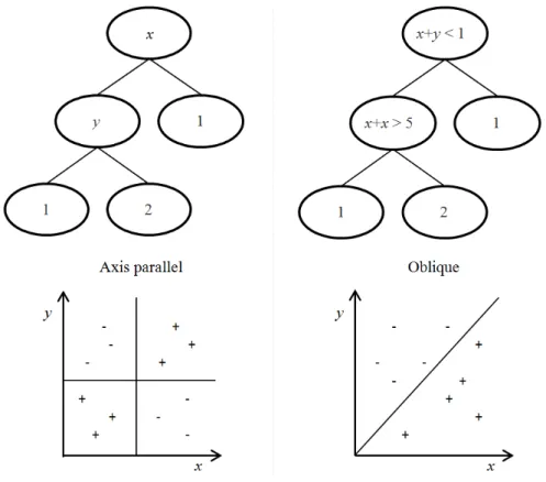
4.1 Axis parallel and oblique decision trees, along with graphs illustrating how the data is partitioned in the two representations. The graphs do not represent the partitioning of the data for the corresponding trees. . . 57

4.2 CheckCondition2Vars, function for an oblique decision tree. . . 59

4.3 Oblique tree used in the study of Shaliet al. [8]. . . 60

4.4 Axis parallel decision tree. . . 61

4.5 An arithmetic tree. . . 62 xii

(14)

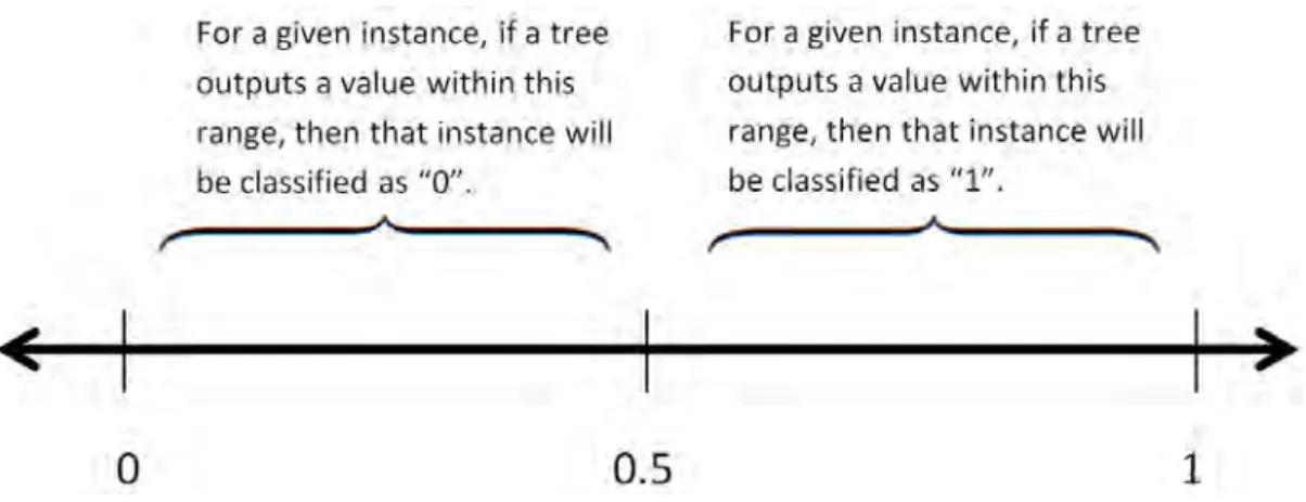
LIST OF FIGURES xiii 4.6 Illustrating how to map the output of a GP tree onto two classes using

a threshold value. In this figure, the threshold is 0.5. . . 63

4.7 An example of a tree created using class enumeration. . . 70

4.8 Representing a categorical attribute as a numerical one. . . 75

4.9 The IN function proposed by De Falco et al. [9]. . . 79

5.1 Difference in the number of attributes and instances in the binary data sets. . . 111

5.2 Difference in the number of attributes and instances in the multiclass data sets. . . 112

5.3 Difference in the number of classes in the multiclass data sets. . . . 112

6.1 Example of a GP tree using a decision tree representation. . . 117

6.2 Intervals created using EWI. . . 118

6.3 Intervals created using GPEI. . . 120

6.4 Illustrating the alter interval GO. The algorithm selected attribute 3 (highlighted in grey) for modification. . . 123

6.5 Illustrating the alter interval GO. The intervals for attribute 3 were altered which resulted in three new intervals. . . 123

7.1 Arithmetic tree representation for GP. . . 127

7.2 Decision tree representation for GP. . . 128

7.3 Logical tree representation for GP. . . 128

7.4 The between GP operator for logical tree representations. . . 129

7.5 Creating the OUT function by preceding the between with a NOT operator. . . 130

8.1 Pruning trees and adding encapsulated terminals at the leaves. . . . 135

8.2 Evaluating a tree with an encapsulated terminal. . . 135

9.1 Illustrating an ensemble. . . 144

9.2 Example of a chromosome created usingSSGA-GP. The genes corre- spond to GP trees which have been added from different GP generations.147 10.1 Ensemble with corresponding trees at each index. . . 153

11.1 Comparing GPEI and EWI in terms of training and test accuracy (%). 166 11.2 Illustrating the average training accuracy (%) for the different representations. . . 170

11.3 Illustrating the average test accuracy (%) for the different representations. . . 172

(15)

11.4 Comparison between the average test results for the ensembles and

standard GP. . . 188

A.1 Main menu. . . 213

A.2 GP Arithmetic Representation menu. . . 215

A.3 Popup message which appears at the end of the run. . . 216

(16)

List of Tables

2.1 Fitness case for the even-3-parity problem. . . 15

2.2 Illustrating fitness proportionate selection. . . 17

3.1 Class output from figure 3.2, and the output for the simplistic classifier. . . 34

3.2 Confusion matrix, extracted from [10]. . . 35

3.3 Illustrating accuracy paradox - classifier 1 confusion matrix. . . 35

3.4 Illustrating accuracy paradox - classifier 2 confusion matrix. . . 35

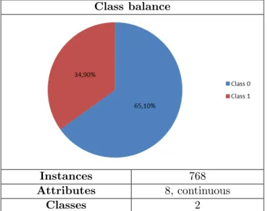
5.1 Pima Indians data set characteristics. . . 100

5.2 Sonar data set characteristics. . . 101

5.3 WDBC data set characteristics. . . 101

5.4 Parkinsons data set characteristics. . . 102

5.5 Mammographic data set characteristics. . . 102

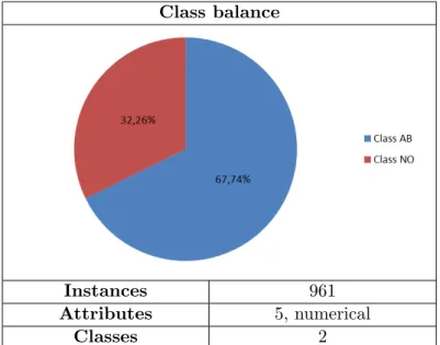
5.6 Ionosphere data set characteristics. . . 103

5.7 Spectf data set characteristics. . . 103

5.8 Climate data set characteristics. . . 104

5.9 Fertility data set characteristics. . . 104

5.10 Monk2 data set characteristics. . . 105

5.11 TTT data set characteristics. . . 105

5.12 Balance data set characteristics. . . 106

5.13 Car data set characteristics. . . 106

5.14 Glass data set characteristics. . . 107

5.15 Ecoli data set characteristics. . . 107

5.16 Zoo data set characteristics. . . 108

5.17 Iris data set characteristics. . . 108

5.18 Wine data set characteristics. . . 109

5.19 Yeast data set characteristics. . . 109 xv

(17)

5.20 Vehicle data set characteristics. . . 110

5.21 Soybean data set characteristics. . . 110

6.1 Sample data for an attribute. . . 119

6.2 Experiments conducted and their different combination of parameters. 124 6.3 Selected data sets for the adaptive discretisation experiments. . . . 124

6.4 GP parameters. . . 125

7.1 Characteristics of the five experiments comparing different GP representations for binary data classification. . . 130

7.2 Selected binary data sets for the GP representation experiments. . . 131

7.3 GP Parameters for comparison of different GP representations for data classification. . . 131

8.1 Data sets used for GP encapsulation experiments. . . 140

8.2 GP parameters used. . . 140

9.1 Selected data sets for the hybridisation experiments. . . 150

9.2 GP and GA parameters for the hybridisation experiments. . . 151

10.1 Possible functions for g(x_i). . . 156

10.2 Different weight values and their corresponding value for g(x_i). . . . 157

10.3 Illustrating how the weights are updated. Let the correct class for some instance of data be “B”. . . 160

10.4 GP parameters used. . . 161

10.5 Data sets used for ensemble construction experiments. . . 162

11.1 Experiment IDs for the discretisation methods. . . 164

11.2 Training accuracy (%) results for the different GP discretisation methods. For each data set, the best result is highlighted in bold, and was statistically tested with every other result. . . 164

11.3 Test accuracy (%) results for the different GP discretisation methods. For each data set, the best result is highlighted in bold, and was statistically tested with every other result. . . 165

11.4 Average size (number of nodes) of the best GP individuals for each method. The smallest size for each data set is highlighted in bold. . 167

11.5 Comparison between GPEI with arity 2 and other state-of-the-art discretisation methods. . . 168

(18)

LIST OF TABLES xvii 11.6 Training accuracy (%) results for the different representations. For

each data set, the best result is highlighted in bold. A “**” indicates that the best result for the data set is statistically significant when compared to that result. A “†” indicates a statistically insignificant result when compared to the best result. . . 169 11.7 Test accuracy (%) results for the different representations. For each

data set, the best result is highlighted in bold. A “**” indicates that the best result for the data set is statistically significant when compared to that result. A “†” indicates a statistically insignificant result when compared to the best result. . . 170 11.8 Variance amongst the different methods for each data set. . . 172 11.9 Average size (number of nodes) of the different representations. The

smallest result for each data set is highlighted in bold. . . 173 11.10Training accuracy (%) results for standard GP and the two proposed

encapsulation methods. For each data set, the best result is highlighted in bold, and the results for the encapsulation methods were statistically tested with the results obtained by standard GP. A “**”

indicates that the result is statistically significant when compared to the result obtained by standard GP without encapsulation. A “†”

indicates a stastically insignificant result compared to standard GP without encapsulation. . . 174 11.11Test accuracy (%) results for standard GP and GP with the two pro-

posed encapsulation methods. For each data set, the best result is highlighted in bold, and the results for the encapsulation methods were statistically tested with the results obtained by standard GP.

A “**” indicates that the result is statistically significant when compared to the result obtained by standard GP without encapsulation.

A “†” indicates a statically insignificant result compared to standard GP without encapsulation. . . 175 11.12Comparison between the number of encapsulated terminals which

were present in the best GP individuals for the two encapsulation methods. All the results obtained by encapsulation with maintained list were statistically significant compared to when the list was not used, this is denoted by “**”. . . 176 11.13Average training classification accuracy (%) for GA-at-end. For each

data set, the best result is highlighted in bold, and the best ensemble result is statistically tested against the standard GP result. . . 177

(19)

11.14Average test classification accuracy (%) forGA-at-end. For each data set, the best result is highlighted in bold, and the best ensemble result is statistically tested against the standard GP result. . . 178 11.15Average training classification accuracy (%). The best result for each

data set is highlighted in bold. The result for each ensemble method was statistically compared to the result obtained by standard GP. Be- tween each pairwise comparison, a “**” denotes that the higher result is statistically significant. A “†” denotes statistical insignificance. . 180 11.16Average test classification accuracy (%). The best result for each data

set is highlighted in bold. The result for each ensemble method was statistically compared to the result obtained by standard GP. Between each pairwise comparison, a “**” denotes that the higher result is statistically significant. A “†” denotes statistical insignificance. . . . 180 11.17Comparison of the average size of the ensembles ofGA-after-each-gen

andGA-with-HC. For each data set, the larger result was statistically compared to the other result. A “**” indicates that the result is statistical larger than the other method. A “†” denotes a statistically insignificant result. . . 182 11.18Training accuracy (%) comparison betweenGA-at-end and other meth-

ods found in literature. . . 183 11.19Test accuracy (%) comparison betweenGA-at-end and other methods

found in literature. . . 183 11.20Training accuracy (%) comparison between the proposed ensemble

methods and other methods found in literature. . . 184 11.21Test accuracy (%) comparison between the proposed ensemble meth-

ods and other methods found in literature. . . 184 11.22Training accuracy (%) results for the different ensembles and standard

GP. The best result for each data set is highlighted in bold. For each data set, ensemble5 was statistically compared to standard GP 200 generations, ensemble 7 to standard GP 280 generations, and ensemble9 to standard GP 360 generations. . . 186 11.23Test accuracy (%) results for the different ensembles and standard

GP. The best result for each data set is highlighted in bold. For each data set, ensemble5 was statistically compared to standard GP 200 generations, ensemble 7 to standard GP 280 generations, and ensemble9 to standard GP 360 generations. . . 187 11.24Training accuracy (%) comparison between the proposed ensemble

construction method and other methods found in literature. . . 189

(20)

LIST OF TABLES xix 11.25Test accuracy (%) comparison between the proposed ensemble con-

struction method and other methods found in literature. . . 189 11.26Comparison between the hybrid ensemble methods with the ensemble

construction methods. The best training and test result for each data set is highlighted in bold. For each training and test set, a “**”

denotes that the best result is statistically significant when compared to the other result, and a “†” denotes statistical insignificance. . . . 190

(21)

List of Algorithms

2.1 Generational GP algorithm. . . 7

2.2 Pseudocode for tournament selection. . . 18

2.3 Steady state GP. . . 23

6.1 Pseudocode for creating an attribute node using GPEI. . . 121

6.2 Alter interval genetic operator. . . 122

8.1 Pseudocode for encapsulation in the context of data classification. . . 134

8.2 Pseudocode of proposed GP algorithm with encapsulation. . . 136

8.3 Pseudocode for initialising the maintained list. . . 137

8.4 Pseudocode for updating the maintained list. . . 138

8.5 Pseudocode which selective encapsulation uses for adding terminals to the GP trees. . . 139

9.1 Pseudocode of genetic algorithm for ensemble representation. . . 142

9.2 Pseudocode for GA mutation. . . 142

9.3 Pseudocode for GA one point crossover. . . 143

9.4 Pseudocode forGA-at-end. . . 145

9.5 Pseudocode forGA-after-each-gen. . . 146

9.6 Modified mutation GA operator. . . 148

9.7 Pseudocode forSSGA-GP. . . 149

10.1 Pseudocode for adding a tree to the ensemble. . . 154

10.2 Pseudocode for evaluating a GP tree. . . 158

10.3 Pseudocode for updating the weights. . . 159

xx

(22)

Chapter 1

Introduction

1.1 Purpose of the Study

Data classification techniques deal with creating classifiers which allocate a label to data. These techniques use the existing data in order to produce these classifiers, and once created, the classifiers are applied to new unseen data. An application area which illustrates the purpose of data mining is the allocation of credit scores to individuals. A credit score represents a numerical value which denotes the risk associated to lending finance to an individual. Assume that a large database containing relevant information about consumers and their credit behaviour is maintained, and that through the use of data classification, a classifier is created. Provided a suitable classifier is created, this could assist credit providers in assessing the risk involved in providing financial support to new customers.

Various techniques have been applied to data classification, including statistical methods such as Bayesian and regression methods, and evolutionary algorithms such as genetic algorithms and genetic programming algorithms. Genetic programming is inspired by nature. It has often been used to solve data classification problems and has been successful in producing good classifiers [11]. Despite the large number of studies which have addressed data classification by using genetic programming, it is apparent from the literature that there are still certain areas of research which have not been explored. These areas represent the rationale behind this dissertation and are listed as the objectives in the following section.

1.2 Objectives

The primary objective of this dissertation is to develop, and evaluate the performance of genetic programming in the domain of data classification, and to investigate certain areas of research which have not been previously addressed. The

1

(23)

objective of this dissertation is not to propose algorithms which will outperform all the existing methods found in the literature, but instead, the objective is to conduct an investigation on how several proposed genetic programming methods perform on data classification problems. Tied in with the primary objective previously stated, this dissertation will conduct a thorough analysis of the related literature on genetic programming and data classification. Five objectives were formulated for this dissertation and are listed below:

• Objective 1: Incorporating discretisation into genetic programming.

To determine and compare the performance of several proposed methods which incorporate discretisation into a genetic programming algorithm. The proposed methods will be applied to data sets in which the attributes are made up of real values.

• Objective 2: Genetic programming representations for binary data classification.

To determine the primary representations for genetic programming and data classification, and to compare their performance in the context of binary data classification.

• Objective 3: Creating an encapsulation genetic operator for data classification.

To incorporate, investigate and evaluate the encapsulation genetic operator in the context of data classification. The objective is to determine whether the performance of a genetic programming algorithm is impacted as a result of incorporating this genetic operator.

• Objective 4: Hybridising evolutionary algorithms for classifier ensembles.

To propose, implement, and hybridise a genetic algorithm with a genetic programming algorithm and conduct an analysis on variations of this hybridisation in the domain of data classification.

• Objective 5: Creating a genetic programming ensemble construction method.

To propose and investigate an ensemble construction method which will create genetic programming ensembles. The objective is to determine how a single ensemble can be constructed using genetic programming.

(24)

CHAPTER 1. INTRODUCTION 3

1.3 Contributions

This dissertation makes the following contributions:

1. Discretisation is required when using decision trees and continuous data. There has been no previous work which has incorporated discretisation into the genetic programming algorithm. The findings of this study reveal that discretisation can be successfully incorporated and that the proposed methods achieve good results when compared to existing discretisation methods.

2. The choice of representation is an important decision to make when implementing a genetic program. There has been no previous work comparing the three major representations for binary classification. The findings of this study show that decision trees provided the best overall accuracy; however, any of the three representations can be used in order to achieve good results.

3. Functions are often used when writing a computer program. The encapsulation genetic operator is used to achieve this purpose in the context of genetic programming. There has not been any previous attempt to investigate the encapsulation genetic operator for data classification problems. It was con- cluded from the results that the encapsulation genetic operator can yield an improvement in accuracy.

4. Based on a thorough investigation of the literature, it was found that ensemble methods produce classification models which obtain better results than non- ensemble approaches. This dissertation proposed four ways for combining a genetic algorithm and genetic programming algorithm in order to improve the accuracy of the classifiers. The proposed methods outperformed the standard genetic programming approach. On certain data sets the proposed methods outperformed other state-of-the-art ensemble approaches.

5. Contribution 4 proposed methods for evolving a population of ensembles. This dissertation made another contribution to ensemble methods by proposing a genetic programming ensemble approach which focuses on creating a single classifier. Weights were associated to the instances of data in order to allocate a level of difficulty to the instances. The findings revealed that the proposed method outperformed the standard genetic programming method. The proposed method further provides an alternative approach to existing boosting algorithms.

(25)

1.4 Dissertation Layout

This section provides a summary of the chapters in this dissertation.

Chapter 2 - Genetic Programming

This chapter provides detailed descriptions about genetic programming, and sets the foundation for this dissertation. Each process within the algorithm is thoroughly described and analysed. This chapter also discusses the strengths and weaknesses of genetic programming.

Chapter 3 - Data Classification

This chapter introduces the concept of data classification and describes the relevant terminology. Previous work on data classification is discussed and details regarding active research areas are provided.

Chapter 4 - Genetic Programming and Data Classification

Discussions regarding previous work which have used genetic programming to solve data classification problems are presented in this chapter. The strengths and weaknesses of applying genetic programming to data classification are discussed.

Chapter 5 - Methodology

This chapter describes how the investigation on genetic programming and data classification will be performed, and how each objective will be met. The data sets are described in this chapter.

Chapter 6 - Adaptive Discretisation for Genetic Programming This chapter presents several algorithms which have been proposed in order to incorporate discretisation into the genetic programming algorithm.

Chapter 7 - Genetic Programming Representations for Binary Data Classification

This chapter proposes an investigation on genetic programming representations for binary data classification.

(26)

CHAPTER 1. INTRODUCTION 5 Chapter 8 - Genetic Programming Encapsulation for Data Classifi- cation

Chapter 8 describes how a proposed encapsulation genetic operator can be used in the context of data classification.

Chapter 9 - Hybridising Evolutionary Algorithms

A description of several algorithms for hybridising a genetic algorithm with a genetic programming algorithm is discussed in this chapter. This chapter focuses on evolving a population of ensembles.

Chapter 10 - Genetic Programming Ensemble Construction

This chapter presents an algorithm for evolving a single ensemble using genetic programming.

Chapter 11 - Results and Discussion

Chapter 11 presents and discusses the results obtained by the investigations proposed in chapters 6 to 10. The proposed methods are compared to standard genetic programming and to other existing methods.

Chapter 12 - Conclusions and Future Work

Finally, this chapter provides a summary of the findings from the research presented in this dissertation, and discusses how the objectives presented in chapter 1 have been met. This chapter also describes future work which will be investigated.

(27)

Chapter 2

Genetic Programming

2.1 Introduction

This chapter introduces genetic programming and provides details and an analysis on the different aspects of the algorithm.

Section 2.2 introduces genetic programming, this is followed by an overview of the generational genetic programming algorithm in section 2.3. When using genetic programming to solve a problem, a representation has to be chosen. Each representation has its own function and terminal set, these two concepts are discussed in sections 2.4 and 2.5 respectively. The tree based representation is discussed in section 2.6. Three initial population generation methods are described in section 2.7, followed by a discussion on fitness in section 2.8. Two parent selection methods are discussed in section 2.9; this is followed by section 2.10 which describes three commonly used operators to generate offspring. Genetic programming is executed until a certain condition is met, and this is discussed in section 2.11. The concept of strongly-typed genetic programming is discussed in section 2.12. Control models are highlighted in section 2.13. The concept of code reuse and modularisation is discussed in section 2.14. Genetic programs suffer from bloat, which is described in section 2.15. Like other evolutionary algorithms, genetic programming has its own strengths and weaknesses; these are highlighted in section 2.16. Finally, section 2.17 concludes this chapter and summarises the critical aspects of the genetic programming algorithm.

2.2 Introduction to Genetic Programming

Genetic Programming (GP) was first introduced by Koza in 1992 [3] and deals with evolving computer programs using biologically inspired methods. Each program is represented as an individual in a population, and each individual competes for

6

(28)

CHAPTER 2. GENETIC PROGRAMMING 7 resources and survival, similar to the analogy of natural species competing for resources such as food. Only the fittest or near fittest individuals survive, and they give birth to new offspring in the hope that these offspring will be able to survive.

The process of giving birth to offspring is similar to the concept of genetic operators (GO) which will be further discussed in section 2.10.

GP is stochastic and random in nature, and thus it cannot be guaranteed that a solution to a problem will be found [1], nevertheless, GP has proved successful in numerous application domains and has been used to create programs which are better than those written by human programmers [2].

2.3 Overview of the Generational GP Algorithm

The generational GP algorithm [2] is presented in algorithm 2.1. The first step is to randomly create the initial population of GP individuals. The size of the population is a user defined parameter. The algorithm proceeds into a loop, and each iteration of this loop represents ageneration. The initial population is evaluated by examining each individual in order to determine if a solution to the problem has been found. If a solution is found, then the algorithm can terminate and output the GP individual which solves the problem. However, if no solution exists within the initial population, the algorithm continues. Four actions are performed during each generation: evaluate the current population, apply the selection methods, apply the genetic operators, and finally update the population.

Algorithm 2.1:Generational GP algorithm.

1 begin

2 Randomly create the initial population.

3 repeat

4 Evaluate the population.

5 Apply the selection methods and obtain parents.

6 Apply the genetic operators to the parents, and create offspring.

7 Replace the current population with the offspring.

8 until a solution to the problem has been found, or a termination criteria is met;

9 end

10 return The best individual from the population

The selection methods are applied to obtain parents for the genetic operators.

Once the parents have been obtained, the genetic operators are applied and the new individuals - referred to as the offspring - replace the current population. In each generation of the generational GP algorithm, the entire population is replaced by the offspring. The new population is then evaluated and the process is repeated

(29)

until one of the termination criteria are met.

Typically, the termination criteria is met when the maximum number of generations is reached, or once a solution to the problem has been found [3]. The algorithm which has just been described is thegenerational control model. This shall be further discussed in section 2.13. The following sections describe fundamental areas which are related to the GP algorithm.

The even-3-parity problem will be used to assist with the description of certain processes of the GP algorithm. This is a boolean problem (which has 3 input variables;x,y, andz) in which the task is to create a solution that can correctly output whether a given string contains an even or an odd number of true values. The value

“true” is represented by a 1, and the value “false” is represented by a 0. Consider the string 000, there are no 1s, thus since there are an even number of 1s, the output is 1. Now consider the string “010”, in this case there is an odd number of 1s, thus the output is 0.

2.4 Terminal Set

GP individuals represent candidate solutions to a problem. The problem will typically have a number of input variables which can be used to solve the problem. In GP, the terminal set [1, 2] is made up of all the variables which are used to solve the problem. The terminal set can also contain constants; these for example can be integers, strings, characters, or floating point values which have some significance to the problem domain.

Ephemeral random constants are also added to the terminal set. Whenever an ephemeral random constant is added to the leaf node of an individual during the GP execution, its value is randomly generated within a specified range, and this value remains unchanged during the entire evolutionary process [1, 3]. For instance, let a be an ephemeral random constant with a range of integer values [−1,1]. Thus, at any point during the evolutionary process, if a is selected from the terminal set, a random integer value in the range of [−1,1] will be chosen for it, and the value will remain fixed for the duration of the GP execution. Thus, it is possible that when terminala is selected numerous times, different values are generated. The type and range of the values for an ephemeral random constant are problem dependent.

Finally, any function with an arity of zero is included. Arity is the number of arguments which a function has [2]; figure 2.1 illustrates different arity values. For example, consider arandom() function which generates random integers. Since such a function has an arity of zero, it would be included in the terminal set. These terminals are found at the leaf nodes in tree structures. In the case of the even-3- parity problem, the terminal set will be made up of the three input variables, thus

(30)

CHAPTER 2. GENETIC PROGRAMMING 9 the set will be {x, y, z}.

Figure 2.1: Illustrating nodes with different arity.

2.5 Function Set

Thefunction set contains all the functions specific to the problem domain which are available to the GP algorithm [2]. Examples of such functions are arithmetic functions, logical operators, loop statements and conditional statements. The function set should be made up of functions which would be useful to the domain. In the case of the even-3-parity problem, since this is a boolean problem, a possible function set would include logical operators, such as{AND, OR, XOR}.

Below is a list of commonly used function sets extracted from [1, 3].

• Arithmetic functions: {+,−,×, /}

• Mathematical functions: {sin, cos, tan, exp, square}

• Logical operators: {AN D, OR, N OT}

• Conditional operators: {If −T hen−Else}

2.6 Tree Based GP

As mentioned in section 2.3, the first step in the GP algorithm is to create the initial population which is made up of GP individuals. These individuals - which are made up of elements from the terminal and function set - need to be represented in some manner. This section will discuss the tree based GP representation.

Trees, also known as syntax trees, are the most commonly used representation for GP, and are made up of one or several nodes. The top most node is referred to as the root, and the bottom most nodes are the leaves. Leaves are usually represented by elements of the terminal set. Tree nodes which are non-leaves are represented by elements from the function set. Trees are commonly output from a pre-order traversal to improve readability; however, they are typically evaluated in an infix order to ensure the correct evaluation of the mathematical or logical expressions

(31)

which are represented by the trees. Figure 2.2 illustrates a GP based tree which corresponds to the mathematical expressionmax(x+x, x+ 3×y).

Figure 2.2: GP tree, extracted from [1].

2.7 Initial Population Generation

Once a suitable representation has been decided upon, an initial population can be created. The initial population is referred to as generation zero. Several methods exist for the creation of the initial population. Three common methods for creating the initial population are the full method, the grow method, and finally the ramped half and half method. Additional initial population generation methods for GP trees were examined by Luke and Panait [12].

In order to maintain genetic diversity no duplicates should be created when initialising the population; this is done in order to represent as much of the program space as possible. Koza describes duplicate individuals in generation zero as

“unproductive deadwood” [3].

If only a small portion of the program space is being represented then the GP algorithm may converge prematurely to a local optimum. However, if a sufficient amount of the program space is represented then there is a greater chance of converg- ing to the global optimum. Incidentally, if the program space being represented is too large, then this can hinder GP’s ability to converge towards the global optimum.

Before the initial population generation is described, the term depth needs to be defined. The depth of a node is the distance from the root node to that particular node. The root node has a depth of 1. Themaximum depth of a tree is the distance

(32)

CHAPTER 2. GENETIC PROGRAMMING 11 - in terms of the nodes - from the root of a tree to the bottom-most leaf. From figure 2.3, the tree has a maximum depth of 4. When creating the initial population for tree structures, a maximum depth must be specified in order to limit the size of the trees when they are created.

Figure 2.3: Illustrating the depth of each node within a tree.

2.7.1 Full method

Each individual created by the full method has the maximum possible size, in the sense that the distance from the root node to each leaf is equal to the maximum tree depth [3]. When creating a tree using the full method, provided that the maximum depth has not been reached, an element from the function set is always selected.

The leaves are made up of elements of the terminal set. By using the full method, the distance between all of the leaves and the root is equal to the maximum depth, and consequently, all the trees in the population have the same depth. In figure 2.4, the tree on the left illustrates the result of applying the full method when creating a tree.

Depending on the arity of the functions, the trees might not all have the same number of nodes. For instance, if the full method is used to create a tree using functions of arity 2, then this particular tree will have less nodes than a tree created using functions of arity 3. Regardless of the arity of the functions, all the leaves within all of the trees will be at the same depth.

A consequence of the full method is that a large quantity of the trees in the initial population will have a similar structure. Consequently, the initial population is less diverse due to the similarity in tree structures. This lack of diversity can result in the GP algorithm searching a restricted area of the program space, and

(33)

thus hindering the performance of the algorithm.

2.7.2 Grow method

The grow method creates trees of different shapes and sizes [3]. When creating a tree using this method, at each depth an element from the terminal set or from the function set can be randomly selected. However, at the maximum depth, only an element from the terminal set can be selected. In figure 2.4, the tree on the right illustrates a tree which was created using the grow method.

This method benefits from the fact that trees of different sizes are created which will result in greater diversity as opposed to the full method. Although the grow method results in greater diversity, the method also suffers from the randomness involved in creating the trees, which is highlighted by Poli et al. [1]. Consider the 6-multiplexer problem; this problem has 6 input variables. In order to solve this problem using a tree representation, all of the variables should be used. It is possible, due to the randomness involved when creating the nodes, that the trees created using the grow method are not sufficiently large enough to make use of all the variables.

Figure 2.4: A tree created using the full method (left), and a tree created using the grow method (right).

2.7.3 Ramped half and half

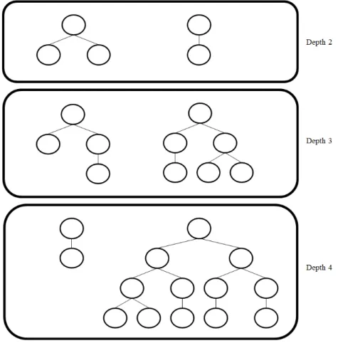
The ramped half and half method creates half of the initial population using the grow method, and the other half using the full method [1]. Let size denote the population size, and letd denote the maximum depth. Thus at each depth, a total of ^size_d−1 individuals are to be created. Of these ^size_d−1 individuals, half of those must be created using the grow method, and the other half using the full method. This method of initial population generation has been proven successful and is commonly used [1]. The reason behind this is that genetic diversity is maintained since trees

(34)

CHAPTER 2. GENETIC PROGRAMMING 13 of different shapes and sizes are created [3].

For example consider a population size of 6 and a maximum depth of 4 which is illustrated in figure 2.5. Half of the population must be created using the grow method, and the other half using the full method. Thus, sincesize = 6 and d = 4 a total of 2 individuals are to be created at each depth. Thus, the individuals are created as follows:

• At depth 2: one tree using the grow method, one tree using the full method.

From the figure, the trees on the left represent those created using the grow method, and the trees on the right were created using the full method. At a depth of 4, the tree created using the grow method is much smaller than the one created using the full method. This is because after the root was set to a function node, the next created node was randomly assigned to an element of the terminal set.

Figure 2.5: Illustrating an initial population created using the ramped half and half method.

(35)

2.8 Fitness

In this section the concept of fitness is introduced. This is an essential part of the GP algorithm and other evolutionary algorithms. The idea of fitness and fitness functions is used to drive the algorithm towards the global optima. These are usually problem dependent formulations and there are a vast amount of approaches present in literature which deal with the concept of fitness in different ways. In this section the fundamental ideas are presented.

2.8.1 Fitness cases

The ultimate goal of an evolutionary algorithm, including the goal of GP is to find a solution to a problem. In order to evaluate an individual in the population,fitness casesare required. The fitness cases represent input and output pairs to the problem domain [2]. For instance, assume GP is used to evolve a mathematical function given some values for the input variables, and their corresponding output value. In this case the input and output pairs are known however, the actual mathematical expression is unknown, and the goal of a researcher would be to create an expression which models the data. In this scenario the input variables and their output value represent the fitness cases.

Banzhaf et al. state that a “machine learning system goes through the training set [or fitness cases] and attempts to learn from the examples” [2]. Hence GP must evolve a program which is able to map the input variables onto the output variables of those examples specified as the fitness cases.

The fitness cases must represent a sufficient amount of the problem domain since GP will evolve solutions which meet as many of these fitness cases as possible. Thus, if the problem domain contains an infinite number of cases, a sufficient amount of these cases must be included, as well as those of particular interest to the problem.

For example, consider generating fitness cases in which GP is being used to create a solution to the factorial problem. For input values greater than 1, the factorial of the input is computed in the same manner. Two particular cases which have to be included in the fitness cases are when the input is 0 or 1, as these both generate an output of 1.

Table 2.1 illustrates an example of fitness cases for the even-3-parity problem.

In this situation the input variables arex,y, and z, and the output variable is also illustrated. Based on the fitness cases in the example, the goal of GP is to evolve an individual which will correctly map the three input variables onto the output variable for each fitness case.

(36)

CHAPTER 2. GENETIC PROGRAMMING 15 x y z output

0 0 0 1

0 0 1 0

0 1 0 0

0 1 1 1

1 0 0 0

1 0 1 1

1 1 0 1

1 1 1 0

Table 2.1: Fitness case for the even-3-parity problem.

2.8.2 Fitness functions

As previously stated, the fitness cases are made up of input/output pairs, however, a numerical measure is required in order to determine how good an individual actually is. In other words, a measure is required to determine how close/far an individual is from a perfect solution, and this measure can be used to compare one individual to another. Fitness functionsare used to obtain afitness value for each GP individual.

Banzhaf et al. define fitness as a “measure used by GP during simulated evolution of how well a program has learned to predict the output(s) from the input(s)” [2].

Additionally, the fitness value is used to determine which areas of the program space are useful in solving the problem [1]. The raw fitness denotes the fitness of GP individuals with respect to the problem domain [3]. Thus the raw fitness for one problem may be different to the raw fitness in another.

Thenumber of hitsis the number of fitness cases for which an individual produces the same output as the fitness cases. In certain cases the raw fitness is equal to the number of hits. From this formulation, the greater the number of hits, the better an individual is.

Since in certain problem domains, a lower raw fitness may represent a better individual, and in other domains, a higher raw fitness represents a better individual;

an alternative measure is to use the standardised fitness. A lower numerical value denotes a better individual when thestandardised fitness is applied [3]. One way to formulate the standardised fitness is to use the raw fitness in the following way: if the problem is a minimisation problem (in which case a lower raw fitness represents a better individual), then the standardised fitness is equal to the raw fitness. However if the problem is a maximisation problem, then a higher raw fitness represents a better individual, and thus the standardised fitness can be formulated asraw_max− raw_{f itness}, where raw_max denotes the maximum possible raw fitness value for the problem [3].

Fitness functions can have either have a single objective, or multiple objectives.

(37)

Fitness functions play an important role in guiding the GP algorithm towards the global optimal solution. The function needs to be correctly defined in such a way so that individuals representing weaker areas of the program space are not confused to be stronger areas and vice versa. Additionally, the fitness function must be able to determine near-solutions as well as solutions to the problem. Examples of fitness functions for solving different problems are listed below:

• In a symbolic regression problem, a suitable fitness function would be the cumulative absolute value in difference between the correct output and the output of the individual across the fitness cases [3].

• In the case of data mining, one could define a fitness function which measures the percentage of instances which GP is able to correctly recognise from the fitness cases [13].

• In solving the artificial ant problem, a fitness function could be one that de- termines the number of pieces of food which has been picked up [3].

• In solving the 11 multiplexer problem, the raw fitness was defined as the number of hits [3].

• In the game Ms. Pac-Man, the fitness function favoured higher scores by adding the scores for the pills, power pills and ghosts eaten [14].

Multi-objective fitness functions are made up of two or more different objectives.

A GP algorithm which implements this approach is referred to as a multi-objective genetic program (MOGP). A MOGP algorithm deals with simultaneously finding optimal solutions in order to meet as many of the objectives as possible [1].

A simple example of a multi-objective fitness function for a maximisation problem is one which computes the number of hits, as well as the size of an individual.

For instance,f itness =raw_{f itness}−tree_size, where tree_size represents the number of nodes within a tree. Thus, GP would favour those trees with a higher number of hits which simultaneously represent smaller trees.

2.9 Selection Methods

Selection methods allow GP to select the individuals - known as parents - which are used to create offspring. There are numerous selection methods; however, this section reviews two common methods, the fitness proportionate and the tournament selection methods.

(38)

CHAPTER 2. GENETIC PROGRAMMING 17 2.9.1 Fitness proportionate selection

Fitness proportionate selection [3] is more computationally expensive when compared to tournament selection as it requires additional calculations to be performed for each individual in the population. Firstly the adjusted fitness has to be calculated. Once obtained, a normalised fitness has to be calculated. The reasons for doing so is that it results in fitness values between 0 and 1, and the sum of all the fitness values adds to 1. The normalised fitness is then multiplied by the number of individuals in the population to determine the number of occurrences of each individual in a mating pool. An individual is randomly selected from the mating pool and is returned to be a parent.

• Adjusted fitness:

a(i, t) = _1+s(i,t)¹

where s(i, t) corresponds to the standardised fitness. The standardised fitness transforms the raw fitness of an individual in such a way that a lower value represents a fitter individual. In the situation where a lower value represents a fitter individual, i.e. a minimisation problem, then s(i, t) = r(i, t) where r(i, t) is the raw fitness.

Otherwise, if the problem is a maximisation problem, then s(i, t) =rmax−r(i, t), wherer_max is the maximum possible fitness for the problem.

• Normalised fitness:

n(i, t) = PM^a(i,t) k=1a(k,t)

where M corresponds to the population size.

Individual Standardised Fitness

Adjusted Fitness

Normalised Fitness

Number of Occurrences in Mating Pool

Tree 1 30 0.03 0.09 0.34 ≈0

Tree 2 15 0.06 0.17 0.69 ≈1

Tree 3 5 0.17 0.49 1.94 ≈2

Tree 4 10 0.09 0.26 1.03 ≈1

Total 0.35 1.00 4

Table 2.2: Illustrating fitness proportionate selection.

Table 2.2 illustrates how the fitness proportionate selection method is applied.

The first step is to compute the adjusted fitness (column 3), and then to compute the normalised fitness (column 4). The number of occurrences (column 5) that each tree will appear in the mating pool is determined by multiplying the normalised

(39)

fitness with the population size, in this case the population size is 4. The number of occurrences are rounded up, and from the example, the mating pool is{tree 2, tree 3, tree 3, tree 4}. Parents are then randomly selected from the mating pool.

A disadvantage of fitness proportionate selection is that an individual with a high normalised fitness will appear several times in the mating pool, and consequently there is a greater probability that it will be selected several times. Furthermore, individuals with a low normalised fitness will never be selected. By selecting the same individual to be the parent, this will result in a loss of diversity due to the fact that the same parents will be used repeatedly. This could further lead to premature convergence.

2.9.2 Tournament selection

Tournament selection [2] is dependent on the tournament size. A subset of individuals is created by randomly selecting individuals from the population; the size of this set is equal to the tournament size. The fitness of each individual in the subset is calculated and the fittest individual is returned. This fittest individual which is returned represents the parent which will then be used to create offspring. The pseudocode for tournament selection is presented in algorithm 2.2.

Algorithm 2.2:Pseudocode for tournament selection.

input :tournament size output: A GP individual

1 begin

2 for i←1 totournament sizedo

3 random individual← randomly select an individual from the GP population.

4 if i= 1 then

5 best individual← random individual

6 end

7 else

8 Comparebest individualand random individual and store the one with the higher fitness tobest individual.

9 end

10 end

11 return best individual

12 end

The tournament size dictates theselection pressure [2]. If the tournament size is small then there is a small amount of selection pressure. The opposite can be said for a large tournament size whereby it results in a greater amount of selection pressure.

(40)

CHAPTER 2. GENETIC PROGRAMMING 19 A large tournament size leads to an elitist GP algorithm which could converge prematurely to a local optimum. Tournament selection is a commonly used selection method. In comparison to the fitness proportionate method, tournament selection benefits from the fact that a selection pressure can be used. If the tournament size is selected correctly, then tournament selection will maintain diversity and additionally drive the GP algorithm towards a solution. Additionally, tournament selection does not require the extra computations involved in calculating the adjusted fitness and the normalised fitness.

2.10 Genetic Operators

Genetic operators (GOs) represent the search operations which are used by the GP algorithm. Koza [3] mentions that if two programs are capable of solving a certain problem to a certain extent, then there are some useful parts within those two programs that contribute to the program’s performance. Thus Koza states that by recombining random parts of the parents the resulting programs may be even better at solving the problem [3].

GOs are used to combine, alter or duplicate the genetic material from the parents to obtain offspring. Typically, the initial population will contain individuals which are not able to solve the problem at hand. GOs are thus applied to these individuals in the hope that they will drive the population towards a solution. Thus the GOs are used to transform the population [2]. These offspring are of different shapes and sizes when compared to their parents. The parents are obtained by a selection method as described in section 2.9.

Each genetic operator can be categorised as being a local or a global search operator. A global search operator allows an evolutionary algorithm to explore different areas of the program space. On the contrary, alocal search operator is one which makes use of exploitation to examine the surrounding areas of the program space in which the evolutionary search is currently situated. GP makes use of the GOs to traverse the program space using exploration and exploitation. The application rate of the GOs will affect the evolutionary process. If a large amount of global search is used, then the GP algorithm will jump to random areas of the program space and may never have an opportunity to converge towards the global optimum. Conversely, if a large amount of local search is applied, then the GP algorithm may end up being stuck in a local optimum and not have an opportunity to explore other areas of the program space.

The three most common GOs are the crossover, mutation, and reproduction operators. Koza [3] presents additional operators (permutation, editing, and deci- mation) which can be applied to GP; however, these will not be examined in further

(41)

detail.

2.10.1 Reproduction

The reproduction operator copies a parent across to the next generation by simply duplicating the individual and making no alterations to it [1–3]. The reproduction operator is a local operator since it makes no alterations to the parent being copied across.

2.10.2 Mutation

The mutation operator [1–3] creates an offspring by mutating a single parent as follows. A mutation point, p, is randomly selected in the parent, and the subtree rooted at the point is removed. A new randomly generated subtree is inserted at pointp. Mutation can cause trees to grow rapidly and thuspruningis used to ensure that individuals do not grow beyond a certain size. Pruning is achieved by replacing any function node at the maximum tree depth with a terminal node. Mutation is a global operator due to the fact that random subtrees are created at the mutation points which can result in a significant difference between the offspring and the parent. Consequently, the mutation operator does not promote convergence. Figure 2.6 illustrates the mutation operator.

Figure 2.6: Mutation operator, adapted from [1].

2.10.3 Crossover

Thecrossover operator creates two new offspring which are formed by taking parts (genetic material) from two parents [3] [2]. The operator selects two parents from the population based on a selection method. A crossover point is then randomly selected in both trees, say point p1 and p2, from tree t1 and t2 respectively. The

(42)

CHAPTER 2. GENETIC PROGRAMMING 21 crossover then happens as follows: the subtree rooted at p1 is removed from t1 and inserted into the position p2 in t2. The same logic applies to the point p2; the subtree root at the point is removed from t₂ and inserted into the place of p₁ in t₁. Figure 2.7 illustrates the crossover operator. Crossover promotes convergence and is a local search operator.

Figure 2.7: Crossover operator [2].

2.11 Termination

Koza states that the GP “paradigm parallels nature in that it is a never-ending process” [3]. This obviously is not feasible, hence the GP algorithm should terminate once a success predicate is met. The success predicate can be defined in different ways however the most common one is to find a solution which has a hits ratio of 100%, i.e. a perfect solution to the problem. The success predicate can be problem dependent [1] and thus defined differently from one problem to another. However in certain problem domains, aiming for a perfect solution is not reasonable, hence once a near-solution is found the GP algorithm can terminate.

(43)

2.12 Strongly-Typed GP

Strongly-typed genetic programming [15] enforces constraints on the nodes within a representation. A type is allocated to the terminals and functions, and consequently, this guarantees that syntactically correct trees are evolved. Strongly-typed GP will ensure that during the initial population generation and application of the GOs, the types of the functions and terminals are respected and not violated. Additionally, strongly-typed GP reduces the size of the program space by limiting the different combinations of functions and terminals [15].

TheIf-Then-Else function is one which requires strongly-typed GP. This function is illustrated in figure 2.8, and each of the three arguments can be assigned a type.

The If-Then-Else function has an evaluation (the If part) and two consequences (theThen andElse parts) which are executed respectively based on the evaluation.

Assume a boolean type is assigned to the If part as illustrated in figure 2.8; as a result of strongly typed GP, the If part should always return a boolean type and this enforcement cannot be violated. Thus variables x and y have to be boolean types.

When applying GOs to strongly-typed GP, it must be ensured that the assigned types are not violated. Thus assume in figure 2.8 that the terminalx is selected as a mutation point, it must be ensured that the new subtree at this point will return a boolean value. If the assigned types are violated, then the trees would be invalid.

Figure 2.8: If-Then-Else function.

2.13 GP Control Models

There are two major control models which can be used when implementing a GP algorithm, a generational control model and a steady-state control model [2]. The models control the population and how they evolve. The generational control model

(44)

CHAPTER 2. GENETIC PROGRAMMING 23 was presented in section 2.