1 University of KwaZulu Natal
THE IMPACT OF EXCHANGE RATE MISALIGNMENTS ON ECONOMIC GROWTH OF THE SOUTH AFRICAN CUSTOMS UNION.
Simiso Msomi 207527293
Supervisor : Christian Tipoy Year: 2015
College of Law and Management Studies, School of Accounting, Economics and Finance.
Thesis submitted in partial fulfilment of the requirement of the degree of Masters of commerce(Economics).
2 Acknowledgments
I would like to thank God Almighty for giving me this opportunity of doing a Master’s degree, for it is not by my own intelligence, prays and glory be to him. This task would have been impossible without assistance offered to me by my supervisor Mr Christian Tipoy, I have learned a lot from him in a short space of time.
I cannot express my appreciation enough to my family for the support they have given to me even when I had to sacrifice spending time with them, because I had to focus on my studies. I dedicate a special thanks to Buyeleni Msomi (my mother) for the sacrifices she made to see me achieve my academic goals, this master’s degree is dedicated to you, mother.
Thanks go to my siblings Sandile, Simo, Zolani and Njabulo. I do not have enough words to explain how I value your presence in my life. Thanks to Nompumelelo Mdletshe for being there when my spirit was low. You had words to give to me so that I could remain focused, when I was excited you had a way of reminding me that I have an objective to meet.
Thanks to my friends I am sorry for not spending time with you, but your support is greatly appreciated, Sanele Gumede, Alpheus Mathe, Fani Jojozi, Simo Chamane, Sikhulile Dlamini, Mthokozisi Ngcobo, Mmeli Nzuza, Mzwandile Mdunge, Nhlanhleni Mdunge and Cebolenkosi Ngwenya.
Thanks to the Vice Chancellor for awarding me a bursary at the beginning for the year and I extend my heart felt gratitude to TATA for awarding me a scholarship. These funds have assisted me greatly this year. I owe a great debt you that I can never repay but I wish these words make you understand that I appreciate your financial assistance.
Thanks to the school of Accounting, Economics and Finance for giving me an opportunity to undertake a research project. The research methodology class that was organised by James Fairbun, Claire Vermaark, Harold Ngalawa, John Hart and Collet Muller was fruitful and it made a great contribution to this project.
Enkosi kakhulu everyone for your help
3 Abstract
The dissertation examines the impact of exchange rate misalignments on the economic growth of five countries in the SACU region: South Africa, Lesotho, Namibia, Swaziland and Botswana, using annual data from 1995 to 2012. First and second generation unit root tests are used in order to take into account the existence of structural breaks and cross-sectional dependence. After determining the existence of a cointegration relationship using both Pedroni (2004) and Westerlund (2007) tests, exchange rate misalignments are computed as a deviation of exchange rates from their long-run determinants; estimated using the Pesaran et al.(1997; 1999) mean-group and pooled mean-group. We found that by using the mean-group estimator, the different currencies are overvalued as suggested by Asfaha and Huda (2002) and Saayman (2007), for both the South African and Botswanan currency. Focusing on the results from the mean group, as this estimator is efficient in the presence of cross-sectional dependence in the data, we assessed the impact of misalignment on economic growth using the system-GMM due to the existence of autocorrelation and endogeneity. We found that exchange rate misalignments are not significant in explaining economic growth, even when controlling for terms of trade and openness.
4 Table of Content
Chapter 1………..………..………5
1.0 Introduction……….……….5
1.1Aims and Objectives……….………6
Chapter 2………8
2.0. Literature Review……….………..8
Chapter 3……….………….………17
3.0. Methodology……….………..………17
3.1. Unit Root testing………..…………...……….17
3.1.1 Testing for cross-sectional dependence………..………..………..17
3.2.1 Levin, Lin and Chu Test (LLC)………..………19
3.2.2 Im, Pesaran and Shin Test (IPS)………..………23
3.2.3 Fisher Type Unit Root Test……….………….………25
3.3 Panel Unit Root Testing Allowing For Cross-Sectional Dependence……….….29
3.4 Pedroni Cointegration test………...31
3.5 A panel bootstrap cointegration test………...39
Chapter 4……….…44
4.0 Real exchange rate and Misalignment………....…………...44
4.1 Estimation Results………..………….50
4.2 Estimating correlation between real exchange rate misalignment and economic growth in SACU………52
5.0 Conclusion……….54
References………..……….55
5 Chapter 1
1.0 Introduction
This dissertation looks at the impact of exchange rate misalignments on economic growth for South Africa, Lesotho, Namibia, Swaziland and Botswana, given the theory that exchange rate could stimulate economic growth. The dissertation also investigates the existence of policy coordination among these countries which is a condition of monetary union.
Exchange rate misalignment is a key variable when predicting future exchange rate shifts and the need of adjustment of exchange rates among countries with less flexible exchange rate regimes. Sustained exchange rate overvaluation may constitute a warning sign of adjustment of relative prices and a possible decline in the aggregate growth rate of the economy, and by the same token, the exchange rate misalignment can be used to influence the performance of the economy (Magyari, 2008).
Researchers, such as Collins et al, (1997), Aguirre et al., (2006), and Rodrick, (2007) have indicated the existence of a negative relationship between exchange rate misalignment and economic growth, implying that currency undervaluation will spur on growth. There also exists some conflicting results, such as those of Magyari (2008).
A common currency requires the existence of one central bank. If each country has its own central bank controlling money supply, there needs to be cooperation between the banks.
Under a common central bank, expansionary or contractionary monetary policy will have an impact on all member countries.
The optimum currency area is characterised by a fixed world price mechanism that is based on a floating real exchange rate, which remains fairly stable even if there is a speculative demand Mongelli (2002). The dynamic equilibrium nature of exchange rates allows reversible movements on exports and imports in competing industries, in an optimum currency area emerging risks of exchange rate is not considerable expensive, cost can be covered at a low cost possible (Mundell, 1961).
The central bank does not engage in monopolistic speculation actions, or optimum currency area permit protection for debtors and creditors which stabilises the economy thereby maintaining long-term flow of capital movement. In recent years, in many geographic locations where countries are within close proximity, the optimum currency area has led to
6 regional integration with the main goal being to unify the region and create a free trade zone (Kamar and Naceur, 2007). Regional integration leads to an increase in interdependence between countries which may in turn lead to contagious crisis outbreaks. To avoid this problem, member states have to coordinate and harmonize their exchange rates and economic policies, as the real exchange rate is an important measure for assessing a country’s competitiveness (see Rodrick 2008; Kamar and Naceur, 2007).
This study examines the impact of exchange rate misalignment on economic growth of Southern African Custom Unions (SACU) countries from 1995 to 2012. The first step compute the real equilibrium exchange rate (REER) using the Behavioural Equilibrium Exchange Rate (BEER) approach advocated by MacDonald (1997) and Clark and MacDonald( 1998). As in Magyari (2008), we use the degree of openness, terms of trade and government consumption, a proxy for the Balassa-Samuelson effect; as the determinants of real exchange rate. The BEER is estimated using panel data cointegration technique. The existence of a cointegration relationship implies the existence of some policy coordination among the countries. Misalignments are then measured as deviations of observed exchange rates from the estimated REER; the latter being constructed using the long-run estimates from the cointegrating equation, and the detrended determinants (detrended using the HP filter).
The impact of misalignments on economic growth is estimated using system GMM, due to the existence of endogeneity. However, we have used the misalignment computed after the mean group, as this estimator is efficient compared to the pool-mean group when cross- sectional dependence exists across units.
There exists a cointegration relationship among the variables implying the existence of some form of macroeconomic coordination between the countries under study. The exchange rate misalignments computed using the mean group estimator indicates that all the currencies are overvalued. However, we have not found the existence of a significant correlation between exchange rate misalignment and economic growth.
According to MacDonald (2000) when exchange rate equilibrium is constructed, determinants of real exchange rate may be undermined. It might also ignore relative activity levels and net foreign assets position. Besides, there are various other methodologies that can be used when one constructs the equilibrium exchange rate. Some of these methodologies are the Fundamental Equilibrium Exchange rate of Williamson (1994) and the Natural Real Exchange Rate (NATREX). The estimated REER may therefore depend on the methodology
7 used. This study does not take also into account the possibility of non-linearity that may exist first between the real exchange rates and its determinants and second, between the variables entering the growth regression. These are some of the limitations of this study.
1.1Research Question and Objectives The aims of this study are:
To establish the existence of macroeconomic policy coordination between the countries;
To compute the exchange rate misalignments in order to determine if currencies are overvalued or undervalued;
To analyse the impact of exchange rate misalignments on economic growth.
Hypothesis of the study Research Questions
Is there macroeconomic policy coordination among the countries under study?
Does currency undervaluation or evaluation stimulate economic growth?
8 Chapter 2
2.0. Literature Review
2.1 Policy Coordination For Regional Integration
Internationally, regional economic integration has become a common phenomenon in recent years. The order of integration begins with weak integration to strong integration, to a free trade zone, a custom union, common market, an economic union and lastly a complete political union.
International trade theory argues that free trade between economies will allow countries to focus on producing goods and services efficiently. Additionally, free trade between countries results in economic growth and brings about foreign direct investment (FDI) inflow through the transfer of technology and skilled labour (Asfaha and Huda, 2002). Regional integration leads to rising interdependence between member states, and is more likely to cause a crisis especially if there is a lack of policy coordination. This was witnessed in the European Union in 1992, and in Latin America in 1994 (Baig and Goldfajn, 1998), and in the last global financial meltdown. To prevent such situations, or to reduce the possibility of running into an exchange rate crisis, member states harmonize their exchange rates and monetary policies (Krugman, 2001). The most advanced stage of coordination between countries is achieved when member states enter into a currency union.
Terra and Valladares (2003) define exchange rate misalignment as deviations occurring around a long-run, real exchange rate equilibrium relationship, and likely to be associated with regime switching thereby allowing for these misalignments to be interpreted as depreciation or appreciation phenomenon. Devarajan (1997) estimates real exchange rate misalignment through using a nominal exchange rate that takes into account price level differences across countries. Aguirre and Calderon, (2005) used bilateral nominal exchange rate for the current period multiplied by domestic price level in the current period divided by foreign current price level.
An increase in regional economic dependence normally generates a need for a regional multicounty currency area, except in situations where it is believed that one country always describes the optimum currency area, implying that political limits and currency borders do not need to be reconciled (Alesina, 2003). There are a series of stages to be followed when creating a single currency among member states, and there should be a period when different
9 currencies are freely exchanged at a constant rate. This is succeeded by a monetary union with a single currency and a single exchange rate, a single monetary market and unrestricted currency movement and deposit at a constant rate (Kamar and Naceur, 2007). When member states are in a monetary union and banking policies are the same, and there is no central bank managing a pool of foreign exchange reserves, financial market integration leads to the convergence of member states’ economies (Buiter, 2000).
Cooper and Kempf’s (2003) model used to implement a single currency provides a very favourable view. With all sovereign countries entering into a single currency requiring strong international commitment, there is no single monetary authority. As has been seen with Spanish Mercado Común del Cono Sur (MERCOSUR), a Latin American regional union, the lack of a real exchange rate and coordination in a regional monetary union, which is accompanied by trade barriers leads to the economic turmoil evident in Brazil and Argentina (Kamar and Naceur, 2007). Monetary policy implementation must be coordinated in all countries seeking to use a common currency because their policies should have a similar impact on the exchange rate, whereas if member states have different monetary frameworks, the result is different impacts on real exchange rate (Frankel 1999).
It is important to measure the extent to which monetary policy affects budget deficits, government expenditure, and trade policy on exchange rate movements on all member states to be able to evaluate if these effects of monetary policy have similar outcomes in all member states (Bayoumi and Mauro, 2001). If it is determined that the effects of monetary policy are similar in all member countries, the successful launch of a new currency among member countries could be expected. Alternatively, if it is determined that the effects of monetary policy on all member states are different, especially policies affecting exchange rate behaviour in each country, it is likely that coordination is not sufficient and hence the launch of a common currency is likely to run into problems. This is a situation where there is still a need for a macroeconomic policy harmonization (Kamar and Naceur, 2007).
The real exchange rate defines a relationship between national and international currency prices. When there are changes in high powered money which causes price levels to change and to be different from the price levels prevailing in the rest of the world, the real exchange rate also changes from that of the rest of the world (Sungur, 2004). Edward (1988) argues that the real exchange rate measures the relative prices of goods and services, precisely.
Stabilisation is not compatible with fixed exchange rates in relation to free capital movements
10 (Christiano et al., 1999). The real exchange rates of countries in the GCC which is fixed against the US dollar, have a monetary policy that is connected to the US monetary policy to minimize the effect of interest rates on the real exchange rate behaviour (Laabas and Limam, 2002).
In the region of GCC countries, which usually experience capital flows as a result of increases in the price of oil, it is reasonable to expect an increase in the stock of net foreign assets, thereby leading to an increase in money supply. This leads to a fall in interest rates resulting in a rise in the demand for money, and giving further rise to the supply of money due to an increase in oil price in the Gulf Cooperation Council countries. This increase in the supply of money creates inflationary pressure because money growth is in double digits for Qatar and UAE, which once went as high as 34% (Laabas and Limam, 2002). Kamar and Naceur, (2007) found on many occasions that money growth in the Gulf Cooperation Council countries converged, and on many occasions in the same period of analysis countries have experienced disparities. Kamar and Naceur, (2007) found that Qatar is not correlated with other countries, and Oman was negatively correlated with only one member country, the UAE. On the other hand EAU was also correlated with Saudi Arabia, and Saudi Arabia was correlated with Kuwait and had a strong positive correlation with Bahrain. They also determined that Kuwait started at a higher level but converged rapidly over a period of two years. Kuwait experienced high interest rates, which later declined to the level of its regional partners (Ramanathan, 2007; Setser and Ziemba, 2009).
The method used to finance a budget deficit is important for determining if inflationary pressure is likely to emerge. If it is financed through taxation or by means of internal borrowing, an economy is exposed to the risk of experiencing depressed private spending offsetting a rise in government spending. If a budget deficit is financed through borrowing from the rest of the world, inflationary pressure may be reduced by increasing the supply of imports. Any form of monetization of debt to GDP increases the degree of inflationary pressure (Sala-i-Martin and Sachs, 1991). But in the Gulf Cooperation Council, a country’s fiscal deficit does not explain their economic situation, the best explanation for this economic event is budget surplus, which can also explain their inflationary pressure. In addition, all funds needed in the Gulf Cooperation Council are financed mainly through oil reserves instead of borrowing or assets’ sales (Setser and Ziemba, 2009).
11 Budget surplus is a result of oil revenue, not because of increased taxes or reduction of government spending; a decrease in net domestic assets is counteracted by an increase in net foreign assets (Sala-i-Martin and Sachs, 1991). In the Gulf Cooperation Council net foreign assets are more important, and can result in even more high powered money causing inflationary pressure. These countries rapidly convert fiscal surplus into government expenditure thereby increasing aggregate demand and offsetting demand-pull inflation.
However, increases in government expenditure can lead to an increase in public servants’
wages, making the private sector, which is competing for employees, increase wage offers and consequently push up inflation. The literature indicates that a negative relationship existing in the budget’s balance in the long-run, means an increase in the budget and results in real exchange rate appreciation Kamar and Naceur, (2007).
Common currency allows liquidity service provided by the central bank to circulate over a large geographic reach as preferred method of payment, store of value and unit of account, common currency give way to clear price transparency thereby preventing price discrimination and encouraging competition. Additionally price stability is realised and there is access to a wider and more transparent financial market, which promotes external financing, which mostly benefits countries that have historically been experiencing inflationary pressure. This is because in the economic and monetary union there are plausible anti-inflationary policies Mongelli (2002). Capital mobility rises because of the increasing degree of openness within countries, resulting in a higher likelihood of fluctuations in capital flow. Economic theory is unclear about the exact effect of commercial liberalization. For Gulf Cooperation Council countries, when there is an increase in the rest of the world’s price of exports, it means for them an increase in the price of oil, which leads to an increase in capital inflow (Setser and Ziemba, 2009).
Magyari (2008) argues that the real exchange rate is an important macroeconomic policy element, mostly for developing states. Here it is used to estimate fluctuations of the future exchange rate for those countries with flexible exchange rates and to determine the need to move exchange rates among countries with less floating regimes. If the exchange rate is sustained, overvaluation may serve as a warning sign for an adjustment of relative prices and the likelihood of a slowdown of the aggregate growth rate of the economy. According to Rodrick (2008) real exchange rate changes also indicate production and consumption taking place between domestic and foreign goods, and a misalignment of the real exchange rate can
12 be used as a method of influencing the actual state of the economy. Countries may try to maintain undervalued economies in an attempt to stimulate economic growth by increasing exports, capital flow and depreciating national currency. This has played a central role in the successful development of China (Coudert et al., 2007).
2.2 Real Equilibrium Exchange Rate: Theory and Methods and Impact of Misalignment on Economic Growth
Purchasing Power Parity is mostly used to determine long-term nominal interest rate, it is given by domestic price level divided by foreign price level. The conjecture forming bases of purchasing power parity is that the law of One Price assumed to be true for every good in the price basket((Rajan and Siregar 2002). The Natural Rate of Exchange rate this approach separate the medium-run and the long-run equilibrium real exchange rate. The medium-run is defined as a period where internal and external balance is achieved, the medium-run is obtained by using current capital stock with foreign debt values whilst the long-term equilibrium is constructed through sustainability of capital stock with foreign debt at a steady state(Egert 2004). The Natural Rate of Exchange rate model does not need a stable equilibrium real exchange rate, and it depends on real economic fundamentals prevailing in the economy(Rajan and Siregar 2002). Behavioural Real Exchange rate is a general approach used to model equilibrium exchange rate, it differentiate between exchange rate, economic fundamentals and short-run variables. Through calculating actual or current misalignment then set short-run variables to zero then substitute into the estimated relationship, misalignment will be the difference between the fitted values and actual values of the real exchange rate(Egert et al 2005). Fundamentals Equilibrium Exchange Rate is concerned with sustainable external equilibrium external account-based equilibrium real exchange rate.
Fundamental equilibrium exchange rate is effective exchange rate that ensures internal and external balance of a country or countries or more simultaneously.
Kamar et al., (2007) explain that it is not easy to set, or determine the most suitable exchange rate, or to keep the exchange rate at the correct level. Some countries seeking to enter into a monetary union, such as the Eurozone, are required to keep their exchange rate floating at a predetermined parity, with approximately 15 percent deviation at most, for a period of two years (Magyari, 2008). Conversion rates to the Euro system determine the extent of the social and financial impact of the Euro changeover, as the rate of changeover must be similar to the rate at which the economy is moving, or the country’s economic performance can be effected.
13 Faced with these situations, it is important to determine a correlation between the growth of the economy and the real exchange rate misalignment (Mastrobuoni, 2004). Existing literature notes that establishing the wrong level of the real exchange rate may cause economic agents to read the economy incorrectly, and consequently create distortions and instability in the economy. Even though this might be true, devaluation of the currency may promote economic growth by increasing exports, which stimulate economic productivity (Bayoumi and Mauro, 2001).
The literature on the impact of real exchange rate misalignment on economic growth uses panel data analysis, although depending on the interests of the researcher, the dependent variables could be real exchange rate misalignment, or economic growth (Rodrick, 2008).
The performance of the indicators included in the studies is considered, as many of these studies use economic growth calculated through the growth rate of the gross domestic product, while in other studies they apply components of the gross domestic product (MacDonald and Vieira, 2010). In the literature many drawbacks have been noticed concerning the real exchange rate misalignment and some research uses purchasing power parity and the approach of the general equilibrium. With these two approaches important drawbacks are noted: for example the purchasing power parity approach cannot be empirically tested because there is not enough data available to permit analysis; and the general equilibrium approach is difficult to use because of specific structural issues in developing countries. Because the approach assumes it is modelling the whole world it is easy to apply (Magyari, 2008; Coudert and Couharde, 2009).
REER equilibrium misalignment estimated for SADC economies reveal continuous overvaluation (Zerihun, 2014). According to Magyari, (2008) there are two studies where real exchange rate misalignment is estimated by a single equation approach. Studies have found the correlation between real exchange rate misalignment and economic growth to be negative, which provides empirical proof that devaluation of a currency can enhance the performance of the economy and economic growth would be higher if new and different channels of transmission were to be found. One of the channels that has been investigated in the literature, is through investment by the rest of the world, as stimulating the accumulation of capital. Alternatively, according to Rodrick (2008) when the real exchange rate moves away from equilibrium it could have an impact on the trade of goods and the competitiveness of the economy with respect to the rest of the world.
14 Kamar and Naceur, (2007) used PMG estimation and found that money supply, budget deficit, government consumption and degree with which countries are involved in international trade had similar effects on the real exchange rate. In addition they determined that if there is misalignment in the short-run, the long run will be characterised by convergence. If there is interdependence between countries it is not appropriate to estimate PMG (Coleman, 2008); this is also shown by Pesaran et al., (1999). Real exchange rates consist of an important characteristic which serves as an appropriate measure for intensity of a country’s international competitiveness (Edward, 1988), while Rodrik (2008) argues either a decline in real exchange rate is an indication that there might have been a rise in domestic costs of production of goods and services.
Real exchange rate misalignment is a function of factors such as openness, ratio of investment to GDP, terms of trade and when there is a rise in explanatory variables it leads to an appreciation of real exchange rates (Eita and Jordaan, 2013). Kamar and Naceur’s (2007) theory shows that the real exchange rate can be influenced by a change of variables, such as monetary policy, government expenditure, terms of trade, degree of openness and capital flows. The real exchange rate has central importance to economic activity since it influences, and it is also influenced by other policies. Achieving policy coordination and harmonization is necessary for successfully establishing a common currency.
Real exchange rate misalignment is more likely to be better explained by panel data, and in situations where there is relatively minor differences between countries on actual real exchange rate and estimated real exchange rate. Misalignment implies that there is a lack of similarity between economies in the explanatory variables of real exchange rates (Dunaway et al., 2006). Empirical work done by MacDonald and Vieira (2010) using a GMM model produces positive estimates for all explanatory variables for real exchange rate misalignment, which means that real GDP growth for their study was influenced by real exchange rate depreciation, and real exchange rate appreciation is found to negatively influence real GDP growth rate. Bleaney and Greenaway (2001) suggest that real exchange rate misalignment has a negative impact on investment; also deviations in terms of trade impact negatively on the economic growth rate. Yotopoulos and Sawada (2006) used panel data when determining that real exchange rate misalignment from purchasing power parity deviations are unique from one country to the next.
15 In literature, the analysis of the exchange rate is done in two parts; undervaluation and overvaluation indicators, for which panel data is used when estimating. When observations are fitted on real GDP growth, it is established that the effect is negative and statistically significant on growth. However, the relationship between economic growth and real exchange rate undervaluation is not statistically significant, but the harmful influence of volatility of exchange rate misalignment is noticeable on economic growth (Rodrick, 2008).
The literature measures real exchange rate misalignment as a deviation from equilibrium real exchange rate (MacDonald and Vieira, 2010). The literature also identifies three different ways that can be used to compare exchange rate misalignment. The first is a PPP-based measure of misalignment, which uses deviations from equilibrium real exchange rate with respect to real exchange rate determined in some year as equilibrium (Magyari, 2008). One disadvantage of using this approach is that purchasing power parity only takes into account changes in the exchange rate resulting from nominal variables, and ignores fluctuations of the exchange rate attributed to real factors.
Secondly, some scholars calculate exchange rate misalignment through differences between the black market and official exchange rates Magyari, (2008). Where a black market premium is used as proxy, it can better explain the extent to which foreign exchange controls may not be explaining real exchange rate misalignment during the time when the rest of the world is moving towards financial integration (Terra and Valladares, 2003). In addition, other studies have found a degree of exchange rate misalignment by the black market premium, and in developing countries in the 1970s and 1980s. Lastly there is a model based on the measure of real exchange rate misalignment; a theoretical equilibrium path in which misalignment is compared by deviations of actual real exchange rates (Aguirre and Calderon, 2005).
The model based measure of real exchange rate misalignment is based on the calculation of equilibrium exchange rate. Establishing real exchange rate equilibrium helps in determining simultaneously internal and external equilibrium. When looking at the literature most empirical work that has been done can be classified in a single equation model, and the general equilibrium simulation method. Both these measures treat real exchange rate as a relative price of traded goods and non-traded, by which it achieves internal and external equilibrium simultaneously (Magyari, 2008). In most instances a single equation method is derived as a reduced form for the equilibrium real exchange rate, basing it on a strong theoretical background (MacDonald and Vieira, 2010).
16 The application of a theoretical framework to derive real exchange rate long-run relationships in the existing literature links the real exchange rate to economic fundamentals, such as terms of trade, trade policy, productivity differentials, net foreign assets among others (Rodrick, 2008). In such situations misalignment happens when there are persistent deviations on real exchange rates from the equilibrium, as well as other factors caused by inadequate macroeconomic traded exchange rate polices (Terra and Valladares, 2003). Aguirre and Calderon, (2005) used a single equation approach to calculate real exchange misalignment.
Initially this was done by estimating a long-run real exchange rate equation using historical data time series, and through panel data techniques. To estimate long-run values of the real exchange rate fundamentals, one can use different kinds of trend-cycle decomposition techniques or one can use a band-pass filter (King and Rebelo, 1993). Magyari (2008) used both HP-filters and band-pass filters.
Atingi-Ego and Sebudde (2004) used the Hodrick-Priscort filter to estimate equilibrium rate exchange rate, which represents a relative stability of existence of real exchange equilibrium.
King and Rebelo (1993) explain that the Hodrick-Prescot filter is used to determine the implicit model that can be filtered to be optimal through minimizing mean square errors.
Ravn and Uhlig (2002) suggest that when conducting a cross country analysis, the Hodrick- Prescort filter parameter should be adjusted according to the forth power of the frequency of observation. Scholars using the Hodrick-Prescott filter are more likely to have different estimations from researchers using differenced data (Cogley and Nason, 1995).
If a researcher is using band-pass filters to estimate equilibrium real exchange rate, estimated coefficients are multiplied with permanent values of the fundamentals. With the other approach used to compute real exchange rate misalignment, we find a difference between the actual and real exchange rate equilibrium (Rodrick, 2008). Alternatively, general equilibrium simulation models can be used to evaluate the behaviour of the real exchange rate. This method is different because the equilibrium real exchange rate meets both internal and external equilibrium conditions. The short fall of this approach is that it ignores important components such as the stock of demand for net foreign assets, but most simulations of this model are based on flow conditions (Magyari, 2008).
With links between real exchange misalignment and economic growth, some literature suggests that real exchange rate misalignment results in a negative effect on the allocation of resources, and therefore economic growth (Bayoumi and Mauro, 2001). However, some
17 researchers hold a premise that undervaluation could be an indication of competitive devaluation that can push exchange rates to a level that encourages an increase in exports (Magyari, 2008). Devaluation positively impacts on the economy because the economy grows through various new sources and adopts new technologies (Terra and Valladares, 2003). Agosin et al. (2012) suggest that there is a connection associated with real exchange rate and an increase with aggregate saving and investment, coupled with a decrease in unemployment, and real exchange rate depreciation, to stimulate economic growth.
18 Chapter 3
3.0. Methodology
The variables used in this study were obtained from the World Bank-Development Indicators data base. For the exchange rate misalignment section, the dependent variable is real exchange rate (REER). The independent variables are given by government consumption (GCON), budget balance (BUDG), degree of openness (OPEN), gross domestic product per capita (GDPPCAP), stock of reserves at the end of the year (RESY). All the variables are in log form except budget balance.
3.1. Unit Root testing
3.1.1 Testing for cross-sectional dependence
It is important to test for cross-sectional dependence, to confirm that it is appropriate to assume cross-sectional independence by Levein, Lin and Chu (LLC), Im-Pesaran-Shin (IPS), Fisher type unit root tests and by the Pedroni cointegration test. If dependence is found, a different unit root test and cointegrating test that allows for dependence must be used to obtain accurate estimates and that would mean we will have to estimate exchange rate misalignment using mean group (MG) instead of PMG. Let us consider a basic panel data regression
where denote the vectors regressors , represents of parameter to be estimated which takes dimension and where denote a characteristic that is fixed across time.
is assumed to be independent and identically identified (i.i.d) across cross-sectional units and over-time period, where the assumption is the null hypothesis . The alternative hypothesis is may be correlated across cross-sectional units, however, the assumption of not autocorrelation remains.
( )
if is generated by correlation coefficient of the distribution and is produced by
19
∑
∑ (∑ ) the resulting number of possible combinations of ( )
If we let be fixed as , to test for Pesaran’s CD test we have to use the Lagrange Multiplier (LM) statistic proposed by Breusch and Pagen (1980) which is also used by Hoyos and Sarafidis (2005) and Pesaran (2012). The statistic is given by
∑ ∑ ̂
where ̂ represents the sample estimate of the pair-wise correlation of the residuals.
∑
∑ (∑ ) where ̂ is estimated of , it is estimated by OLS using the regression
̂
The LM follows a chi-square distribution and it is asymptotically distributed. It consists of degrees of freedom that are described by with the application of the null hypothesis of interest. The LM statistic is not correctly centred when T is finite while N is larger and the bias gets worse as with finite T, this argument is also affirmed by Baltagi et al (2007). The LM test is valid when N is small and T is sufficiently large. Under the null and the LM following a chi-square distribution ̂ with ̂ are asymptotically independent, therefore the scale version if appropriate to use to test the hypothesis of cross dependence even in situations that consist of large N and large T.
√
∑ ∑ ( ̂ )
20 Under the scaled versing of the with the null with while at the same time , , is not correctly cantered at zero. To correct this distortion we use the test proposed by Pesaran (2004)
√
(∑ ∑ ̂
)
In the model above under the null hypothesis of no cross-sectional dependence even for and sufficiently large, this statistic is unlike the LM statistic CD has a mean of zero for fixed values of T and where there is a large panel size, including heterogeneous models non-stationary and dynamic models. When testing for cross-sectional dependence we use critical values on the paper published by Pesaran (2004).
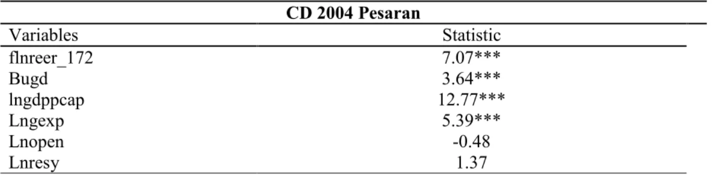
Table 1 presents the result of the cross-section dependence test using the Pesaran (2004) CD test. Openness and stock of reserves shows independence while the remaining variables indicate that dependence exists between the cross sections. Therefore, it is necessary to take into account the existence of cross-sectional dependence while testing for unit root and cointegration.
Table 1 Cross-section Pesaran (2004) Dependence test
CD 2004 Pesaran
Variables Statistic
flnreer_172 7.07***
Bugd 3.64***
lngdppcap 12.77***
Lngexp 5.39***
Lnopen -0.48
Lnresy 1.37
This is a test for cross-sectional dependence. Null hypothesis is cross sectional independence.
.*, **, *** denote significance at 10%, 5% and 1%.
21 3.2.1 Levin, Lin and Chu Test (LLC)
The LLC test states that each unit root has less power against alternative hypotheses, which have consistently higher deviations from equilibrium. This test is more powerful than testing for individual unit root test for each cross-section (Hlouskova and Wagner, 2006).
The LLC test was first proposed by Levin and Lin (1992, 1993) and later by Levin, Lin and Chu (2002). If we observe variables in countries and for periods, and initially we consider a model with individual fixed effect and no time trends, the model consists of a lagged dependent variable which is homogenous by restriction for all individuals of the panel
∑
Where and where . The errors by assumption are independent across all cross-sectional units in the sample. In specifying this model the interest is on testing the null hypotheses against the alternative hypotheses for all applying the auxiliary assumption about the individual effect for all under the null hypotheses . The alternative hypothesis is restrictive because it implies homogenous autoregressive parameters across all panels. In cases where we use the LLC to test for the convergence hypotheses in growth models, the alternative restricts every country to converge at the same rate. Although it is important to understand that using pooled estimator ̂, even when DGP is not identical, does not mean that the unit root test is inconsistent. (Baltagi, 2008).
To illustrate this point, let us consider a sample linear model suppose is equal to 0 in one of the samples and it is equal to 1 in the other half of the sample, assuming that we want to test for the null hypotheses for all the units. This test is possible in the context of pooled estimate ̂ on the entire sample (Baltagi, 2008). Hurlin and Mignon (2006) state that the pooled OLS would produce estimates that converge to 0.5 and the standard error would converge to zero, which means the null hypothesis will be rejected. Normally it is likely to obtain a more powerful test by splitting a sample into two separate parts and then conducting a test with the null hypothesis in both parts (Hlouskova and Wagner, 2006).
Therefore it is important to split issues of estimating the value of the autoregressive parameter to be able to estimate the rate at which convergence is taking place,.
22 The null hypothesis is that all panels contain unit root against the alternative which is all panels contain unit root. The maintain hypothesis is that
∑
Where is denoting the vector of a deterministic trend variables and denotes the corresponding vector of coefficient of the model . In a more specific definition
, and The lag order is not known. Baltagi (2008) argues that LLC suggests a three step approach to be followed when implementing the test. The first step in running the LLC as we need to perform a separate augmented Dicky- Fuller regression for all cross-sections individually (that is equation 4) the lag order is allowed to differ across all individual cross-sections. Given the size of , we choose the largest number of lag order and take the estimated t-statistic of ̂ to evaluate whether a smaller lag order if accepted to a larger order, (t-statistics are normally distributed with a mean of zero and a variance equalling on) the null hypotheses , in both situations when and
Once the adequate lag order is determined, two auxiliary regressions are regressed to obtain orthogonalized residuals:
and ̂ and ̂
The residuals are standardized to control for differences of variances across , ̂ ̂ ̂ and ̂ ̂ ̂ . ̂ denotes standards error from each of the ADF regression, for . The next step is to estimate the short-run and the long run ratio of standard deviations, where the null hypothesis of a unit root for the long-run can be estimated in the following format
̂
∑
∑ ̅
̅
[ ∑
]
where the truncated lag is denoted by ̅ (in this study there is no truncation because data was available for all years) which might be dependent on data. ̅ is estimate in a way that
23 guarantees ̂ is consistent. In each of the cross-section , ̅ ̅ , where the ratio showing the long-run standard deviation to the innovation standard deviation is given by ̂ ̂ ̂ . The estimation of the average of standard deviation is given by ̂ ∑ ̂ . Then to conduct a panel test statistic requires that we run the pooled regression.
̃ ̃ ̃
Based on a given ̃ observations where ̃ ̅ . ̃ denotes the number the average number of each individual in the panel with ̅ ∑ , where ̅ is defined as the average lag order of each individual ADF regression. The common t-statistic for the null hypotheses for, is defined by ̂ ̂ ̂
where;
̂ ∑ ∑ ̃ ̃
∑ ∑ ̃
̂ ̂ ̂ ̃ *∑ ∑ ̃
+
and
̂ ̂
̃∑ ∑ ( ̃ ̃ ̃ )
This equation is to show how the variance is estimated, the adjusted t-statistic is defined by, ̃ ̃ ̃ ̃ ̂ ̂ ̃
̃ The mean and standard deviation adjustments are denoted by ̃ and ̃, is said to be distributed asymptotically . The asymptotic condition requires √ , in this case highlight the situation where the cross-sectional dimension is assumed to be an arbitrary monotonically rising function of (Hlouskova and Wagner, 2006). According to Baltagi (2008), this is applicable to micro panel data for a situation where the pace of the growth of is allowed to be slower than the pace of growth of . Other speeds of
24 divergence are sufficient, but not necessary such as and constant. It is determined above that when using the LLC approach it is required that we specify the number of lags that we are going to make use of in each individual cross-section. ADF regression , and kernel choices are used in the computation of .
We specify an exogenous variable that is going to be used in the test equation, where we can regress an exogeneous plus a trend, or exogeneous variable with no trend or no trend and no constant. When conducting panel unit root testing the acceptable size of is between 10 and 250, and the moderate size for is between 25 and 250. Baltagi (2008) remarks that it might be difficult to compute the standard panel procedures or it may not have enough power for a panel of this size. Although for a very large , when testing for individual unit root time- series, the test will have enough power to apply for each individual cross-section, therefore for a very large and small the usual panel data procedures are preferred (Hurlin and Mignon, 2006). The use of a Monte Carlo simulation conducted by LLC shows that if data is normally distributed a better approximation of empirical distribution of the t-statistic occurs, even in a situation of relatively small sample size. Additionally the panel unit root test provides considerable increase in power compared to a separate unit root test for each of the cross-sections (Hoang and McNown, 2006).
The proposed LLC test like all other approaches is not without limitations. The validity of the LLC test depends on the independence assumption in the entire cross-section and the test is invalid if cross-section correlation is present. Additionally there is a restrictive assumption of all cross-sections do not or contain unit root. Hoang and McNown (2006) argues that with LLC if correlation is present in the cross-section, the test suffers from dramatic size distortion among contemporaneous cross-sectional error terms. Therefore it is important to control for cross-sectional dependence when running panel unit root testing of exchange rate.
3.2.2 Im, Pesaran and Shin Test (IPS)
We have determined from above that Liven, Lin and Chu is a restrictive test that requires to be homogeneous across . The LLC test is suggested to be most suitable for testing for convergence in growth among countries, but the disadvantage of this test is that the alternative is restrictive; it restrict countries to converge with the same rate (Baltagi, 2008).
On the other hand the IPS permits heterogeneous coefficient of thereby introduces an alternative testing approach that is based on the individual unit root test statistic. The IPS
25 argues that the average of the ADF test used when testing contains autocorrelation (Canning and Pedroni, 2004), and for the model has different autocorrelation properties for all cross-sectional units,
∑
As we have seen previously the null hypothesis is that all panels contain unit root, for all cross-sectional units , against the null hypothesis give way for some, but not all, of the individual series to have units roots, which is;
{
This test requires that the fraction of the individual time series that are stationary should not be zero, where . This requirement is important because it ensures we obtain consistency when testing the panel for unit root test (Hoang and McNown, 2006). The t-bar statistic for IPS is defined as the average of the individual ADF statistic;
̅ ∑
where denotes the individual t-statistic for conducting a null hypothesis test, for all in (9). In such situations the lag order is always zero for all ), the IPS offers simulated critical values for ̅ for a different number of cross-sections and number of time series where a Dickey-Fuller regression with ta constant or constant and deterministic trends. The most common use is where the lag order might not be zero for some of the cross-sections, the IPS indicates that an adequately standardized ̅ contains an asymptotic distribution (Hlouskova and Wagner,2006; Baltagi 2008). Supposed we start from a commonly known results time series with fixed
t i ∫
*∫ +
26 as where ∫ represents a Weiner integral that has augmente d supressed in equation (11) (Billingsley, 1961). IPS operate under the assumption that i.i.d and consists of a finite mean and variance. Therefore,
√ ( ∑ ∑ [ ])
√ ∑ [ ]
as we apply the Lindeberg-Levy central theorem, so
√ ( ̅ ∑ [ ])
√ ∑ [ ]
sequentially as followed by , the values given by [ ] and by [ ] are produced by IPS through simulation for different values of and ‘s.
The Monte Carlo simulation reveals that when the lag order chosen is large enough for the ADF regression under consideration compared to a small sample performance of the t-bar test, IPS is reasonable satisfactory and generally better than the LLC test we have seen above (Hoang and McNown, 2006; Hlouskova and Wagner,2006; Billingsley,1961).
3.2.3 Fisher Type Unit Root Test
As mentioned previously the unit root test for panel data is based on a heterogeneous model and includes testing the significance of the result from independent individual test. We have seen that the IPS test uses an average statistic, or we can use the alternative testing approach which is conducted by joining together the observed significant levels of the individual tests. This approach has a strong historical background and is based on the p- values, let us consider equation assumed to be heterogeneous model. The hypothesis is similar to the one we have above,
for all and the alternative hypothesis is for and for with . To illustrate the idea of the Fisher type test we consider the pure time series unit root test statistic, for continuous statistics, the corresponding p-values are denoted by which are uniform variables (0,1) (Maddala and
27 Wu 1999). Since we make an important assumption that there is cross-sectional independence, defined as
∑
The test follows a chi-square distribution comprising of degrees of freedom as for a given value of . This test is simple and provides a robust statistical alternative. Sample size and lag length render this approach extremely favourable to use for panel unit root testing. When we have a large sample, Hurlin and Mignon (2007) suggest this standardised approach is used.
√ [ ]
√ [ ]
∑
√ They argue that this test statistic is consistent with the standardised cross-sectional average of individual p-values, hence the Lendeberg-Levy theorem is sufficient to show convergence to the standard normal distribution in the case of the unit root hypothesis (Hoang and McNown, 2006; Hlouskova and Wagner, 2006).
Billingsley (1961) states that the central limit theorem proposed by Lendeberg and Levy state that if is i.i.d order of white noise variables that has finite second moments, which makes the distribution of ∑ follow the normal distribution with a mean of zero and the variance , with the assumption that . The assumption of independence would be weakened under these conditions.
If we let to be stationary, and allow a positive recurrent aperiodic case of the stochastic process such that it produces which is finite and (16) with a probability of one, and then ∑ is distributed in a way that approaches the normal distribution with a mean equalling zero and variance (Hlouskova and Wagner, 2006).
Condition (16) satisfies the requirement that the partial sums ∑ create a martingale. To make this theorem hold assume that Ω denotes the Cartesian product representing the order of
28 copies of real line, represented by the integers . The coordinate variable is indexed by , the Borel field is denoted by β and the is the likelihood that estimate the finite-dimensional distributions introduced by initial processes (Hoang and McNown, 2006;
Hlouskova and Wagner, 2006). If we suppose that is the Borel field given by { }, through condition (16)
, (17) with a probability of one for integers . If
and where , where is the translation operator (in times series we refer to this as the lag operator), therefore it becomes simple to show that,
. Since is a random process that time averages of a single sequence of events therefore it is consistent with the ergodic theorem. Condition (18) ∑ assumed to have a probability of one. If , let for all values of , where is the value such that it is and , in addition we allow . Because of condition (19) it is determinable that ∑ moves away ( i.e. does not) converge with a probability equalling unity, making and other variables to be adequately defined (Billingsley, 1961). A common premise of renewal type used in equation (19) indicates that
Therefore
{ |∑
| }
If we are able to obtain , where is defines the Markov process satisfying { }, additionally when is finite in the case when contains a stationary distribution. This argument can be supported by showing that ∑ is asymptotically normal whether or not the distribution of is stationary
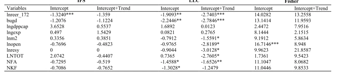
Table2 below presents the results for unit root testing using IPS, LLC and Fisher tests type.
The IPS shows that all variables are insignificant at all levels except for the log of real exchange rate which is significant at 1% level of significant when there is no trend or constant. When a constant and trend is included all variables are insignificant, therefore these variables contain unit root.
29 When using the LLC with trend and no intercept, log of real interest rate is significant, and the government budget balance is significant at 5%; net capital flow and net foreign assets are significant at 10%. When a trend is included, all variables are insignificant. We therefore conclude that these variables have unit root.
For the Fisher unit root test, openness is said to be stationary while using the intercept only.
However, when we consider the intercept and trend option, all the variables contain a unit root.
30
Table 2 Unit root test IPS, LLC and Fisher type test
IPS LLC Fisher
Variables Intercept Intercept+Trend Intercept Intercept+Trend Intercept Intercept+Trend
lnreer_172 -1.3240*** -1.359 -1.9093** -2.7403*** 14.0282 13.2558
bugd -1.2076 -1.1224 -2.2446** -2.7846*** 13.1414 11.9593
lngdppcap 3.6528 0.5537 1.6892 0.0123 2.4472 7.9516
lngexp 0.497 1.5429 0.0821 0.2765 8.1444 2.1515
lnm2 0.3356 0.3851 -0.7912 -1.5591* 9.1912 5.8634
lnopen -0.7696 -0.4823 -0.9765 -2.8189* 16.7146*** 8.948
lnresy 0 0 -0.9044 -3.0128* 9.9623 21.8587
LNTOT 2.0742 -0.4407 0.7365 -2.7605* 1.7361 9.5423
NFA -0.7295 -0.519 -1.4588* -1.6526** 11.1047 8.0682
NKF -0.7086 -0.7652 -1.3028* -1.2479 11.0446 9.8533
Note: LLC, IPS and FISHER statistics correspond to a test of the null hypothesis that all the panels contain unit roots against alternative. *, **, *** denote significance at 10%, 5% and 1%. 2 lags were used to compute the test statistic.
31 3.3 Panel Unit Root Testing Allowing For Cross-Sectional Dependence
To deal with the problem of cross-sectional dependence the test explained above considers a one factor model, with a heterogeneous loading factor for error terms. The test estimates the ADF model consisting of cross-sectional average of lagged and they are integrated of order one as individual series (Breitung, and Das 2005). If there is no serial correlation of residuals the regression is described in the following way
̅ ̅
where we define ̅ ∑ and ̅ ∑ , let denote the test statistic obtained from estimating by using OLS. Unit root testing is now based on cross- sectional units root test ADF statistics (CADF) (Bailey et al, 2014). Pesaran (2003) contends that under extreme cases some values of T may be truncated to avoid having a small value of T in a sample. It follows that we are now able to construct a suitable version of the IPS t-bar test that is able to account for dependence. The modified t-bar is based on a CADF average of individual statistics (see Hurlin and Mignon, 2006). The cross-sectionally augumented IPS is defined as
∑
Under extreme situations a truncated CADF statistic is described in the following way;
,
where and represent intercepts that are fixed to increase the likelihood that associated with [ ] is close to unity. For this paper we are not going to truncate the time because the sample consists of the data starting from 1995-2012, while there are only 5 cross- sectional units. However it is worth noting that truncated data is characterised by a similar asymptotic null distribution that does not depend on the loading factor (Breitung and Pesaran 2008). We use simulated critical values for CIPS with two lags chosen by the SIC.
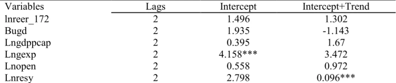
Table 3 shows the results for panel unit root testing while allowing for cross-sectional dependence using the Pesaran (2007) CIPS test. Two lags which were chosen by the SIC.
32 Under the null hypothesis, the series contains a unit root and we can see that when we include an intercept with no trend, log of government expenditure, lag 2 is significant at 1% level of significance. Therefore we reject the null hypothesis that the series contains a unit root. The CIPS test is generating insignificant results for all variables for all lags Bugd, lngdppcap, Lnopen and Lnresy are insignificant at all conventional levels of significance, and the null hypothesis cannot be rejected. lnreer_172 is insignificant at all levels of significance it can be concluded that the series contains units roots.
If we include a constant and a trend, Lnresy is significant at 1% level of significance 2 lags the null hypothesis can be rejected and we conclude the series contains unit root. However, the variables lreer_172, Bugd, lngdppcap, lngexp and lnopen are insignificant at all conventional levels of significance, and the null hypothesis of the series contains unit root.
The results have not changed in any considerable form from those produced by the unit root test that are unable to account for dependence between countries, but it is clear they are slightly different with reference to the log of real exchange rate the under the IPS and LLC, where they were significant. When using CIPS we find that the variable is insignificant; LLC, IPS and Fisher type are not able to detect structural breaks, and if there has been a structural break the power of these test is reduced. Hong and McNown, (2006) affirm that the power of LLC and IPS is low if there is a structural break.
Table 3 Panel Unit Root test (CIPS) Pesaran (2007)
Pesaran (2007) Panel Unit Root test (CIPS)
Variables Lags Intercept Intercept+Trend
lnreer_172 2 1.496 1.302
Bugd 2 1.935 -1.143
Lngdppcap 2 0.395 1.67
Lngexp 2 4.158*** 3.472
Lnopen 2 0.558 0.972
Lnresy 2 2.798 0.096***
This is a test that the null hypothesis of the series contains unit root. The CIPS test assumes that there is cross-sectional dependence in the form of a single unobserved common factor.
.*, **, *** denotes significance at 10%, 5% and 1%. Only results on 2nd lag presented.