Anura Hiraman, Serestina Viriri and Mandlenkosi Gwetu, Efficient region of interest detection for liver segmentation using 3D CT scans, IEEE International Conference on Information Communications Technology and Society, Accepted November 2018. Anura Hiraman, Serestina Viriri and Mandlenkosi Gwetu, Liver CT- scanning using 3D scans, Image Analysis & Stereology Journal, (submitted).
Introduction
Abdominal slices constitute an interesting area of the liver, as these slices contain liver tissue. In addition, the slices of the region of interest are processed by CNN to locate and segment the liver.
Motivation
Segmentation of the liver from these CT scans plays an important role in examining liver functions and can aid in the diagnosis of liver diseases. Segmenting the liver can reduce the computational time required for the analysis, as the liver only occupies part of the abdominal CT scan.
Problem Statement
Despite many years of research and applications of new methods and techniques, liver segmentation remains a challenging task implying that there is still room for improvement of existing models. Liver segmentation is also used for volume measurements used to determine abnormalities of the organ.
Research Objectives
Contributions of the Dissertation
The effect of deeper networks, multi-layer networks, have been investigated to determine whether they perform better than networks with fewer layers.
Organisation of the Dissertation
Conclusion
Introduction
Liver and CT
Liver Anatomy
More than 500 body functions have been associated with the liver and some of them include regulating most chemical levels in the blood, excreting bile and filtering blood coming from the digestive tract [9]. The left and right lobes are the largest lobes and the right lobe is about five to six times larger than the tapered left lobe.
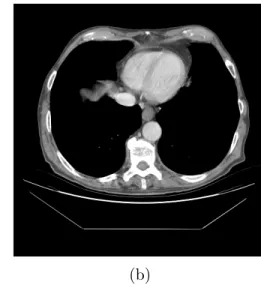
Liver in Abdominal CT image
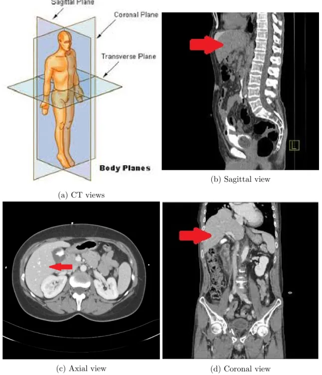
The caudate lobe extends posteriorly from the right lobe and wraps around the inferior vena cava while the quadrate lobe is inferior to the caudate lobe and extends posteriorly from the right lobe and wraps around the gallbladder [8]. The CT scan of the abdomen can be viewed from the axial view, sagittal view, or coronal view.
Related Work
Overview of Literature Review Method
The inclusion criteria include studies conducted in English, liver segmentation methods, liver segmentation using deep learning techniques and only liver segmentation from the 3D medical imaging modalities. Liver segmentation methods Segmentation methods of other organs Liver segmentation used Segmentation of other organs used.
Slice Alignment
The first phase of the SLR is the definition of the research objectives in Section 1.4 of Chapter 1. This method aligns the slice by minimizing the distance between the contours of the images.
Liver Region of Interest Detection
The first step is a rigid registration of the acquired slices to a model that locates the fetal head to estimate the motion parameters. The convolutional neural network is used to detect the presence of the anatomical structures of interest in axial, coronal and sagittal slices extracted from the medical 3D image.
Liver Segmentation Methods
This work used the 2007 MICCAI-SLiver dataset. The quantitative evaluation of the segmentation results showed that the proposed method performed accurately and efficiently. The first stage is a crude extraction of the liver based on MAP estimation and involves four steps.
Conclusion
The distance transformation is calculated and the distance map results are inverted, which is interpreted as a height map. After the initial graph segmentation, five cases have an overlap error of more than 10% and the overall average overlap error is 14.3%. After using the chunk-based refinement method, the average overlap error was reduced to 6.5%, and after using the simplex mesh refinement, it was further reduced to 5.2%.
Introduction
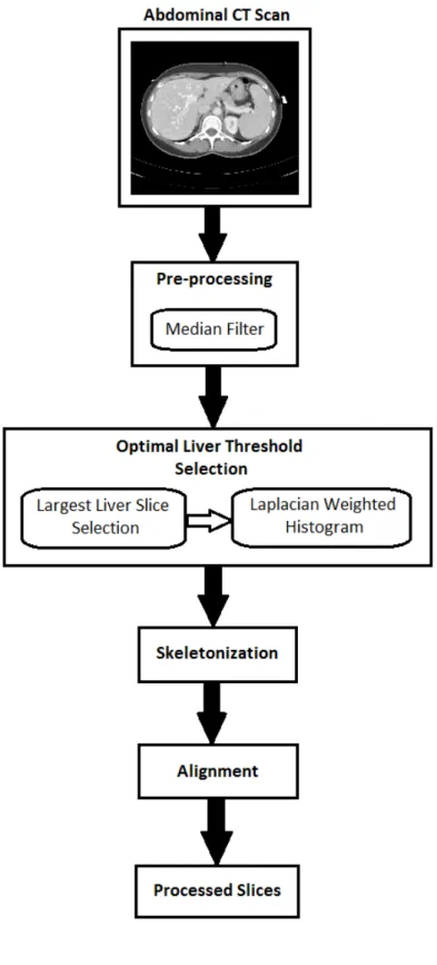
Methodology
- Pre-processing
- Optimal Liver Threshold Selection
- Skeletonization
- Alignment Algorithm
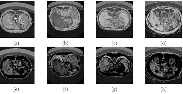
The methodology presented in this article uses this method to determine the optimal threshold value for the liver tissue in a portion of the volume. The global minimum Gmin of the normalized histogram corresponds to the most dominant material transition, in this case the liver tissue. The algorithm does not iterate through the segments of the volume from one end to the other.
Conclusion
The algorithm iterates the list of slices and estimates a warp matrix to be applied to each slice. The list of neighbors is used as a series of reference images to estimate a warp matrix for the floating image. The next chapter describes the liver region of interest detection method that implements CNNs to classify 2D slices to determine a region of interest for liver segmentation.
Introduction
Convolutional Neural Networks
Small Network
Deep Network
Then, a max-pooling layer with a step size of two pixels is used to generate 32 feature maps. After that, a maximum-pooling layer with a step of two pixels is used to generate 64 feature maps. This is followed by a maximum-pooling layer with a step size of two pixels used to generate 128 feature maps.
Data Augmentation
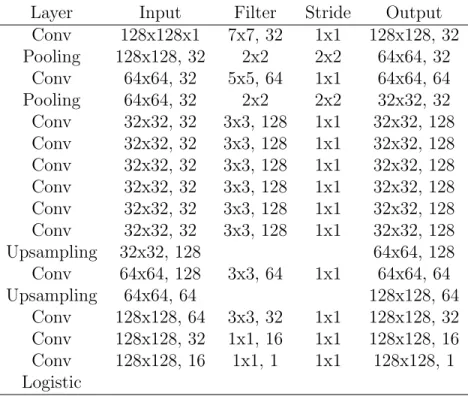
This is then followed by three convolutional layers containing 32 feature maps each and each feature map is connected to all the feature maps in the previous layer by means of 3 x 3 filters. This is followed by two convolutional layers with 64 feature maps each where each feature map is connected to the feature maps in the previous 3 x 3 filter layer. The last convolutional layer has 128 feature maps where each feature map is related to the features in the previous layer by means of 1 x 1 filters.
Training
Where y is the transformed image, x is the original image, b represents the shift in height, rotation angle or shear factor, and W represents the zoom range.
Methodology
- Pre-processing
- Classification of Abdominal and Pelvic Slices
- Classification of Abdominal and Chest Slices
- Post-processing
When training is complete, the network captures a 2D CT slice as a 128 x 128 image and generates a probability that the image is a slice of the abdomen and a probability that the image is a slice of the pelvis. Images that contain evidence of a pelvic ring will be classified as a pelvic cut, and those without it as an abdominal cut. After training, the network takes a 2D CT slice as a 128 x 128 image and produces a probability that the image is an abdominal slice, as well as a probability that the image is a slice containing the thoracic cavity.
Conclusion
Introduction
Pre-processing
Liver Location and Segmentation
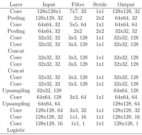
- Network Architecture of Model 1 (CNN without con- catenate layers)catenate layers)
- Network Architecture of Model 2 (With concatenate layers)layers)
- Data Augmentation
- Training
Then, a max-pooling layer with a step size of two pixels is used to generate 64 feature maps. The second convolutional layer contains 64 feature maps and each feature map is linked to all feature maps in the previous layer using filters of size 5 x 5. The ninth convolutional layer contains 64 feature maps and each feature map is linked to the previous layers feature maps with 3 x 3 filters.
Post-processing
Thresholding
Denote that θ is the set of all the parameters, including the filters and softmax parameters of the CNNs. After the training is completed, the trained convolutional neural network is used to predict a liver probability map from a 2D slice, thereby locating and segmenting the liver.
Largest Component Selection
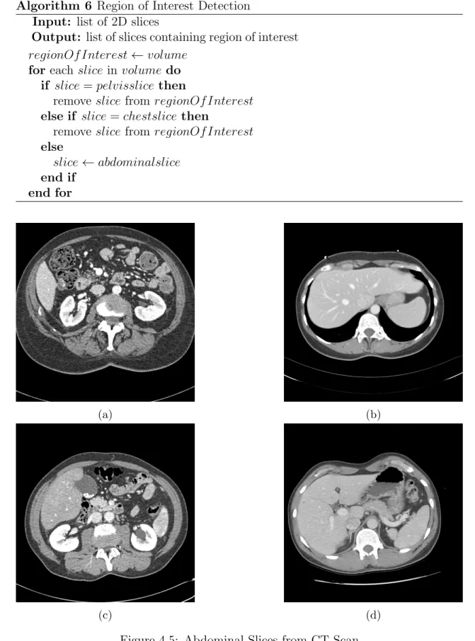
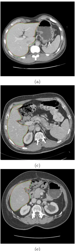
The volume of each component is calculated and the component with the largest volume is selected. The result of the largest component selection can be seen in Figure 5.5, where 5.5(a) and 5.5(c) are images before largest component selection and 5.5(b) and 5.5(d) are their respective results after being processed. Input: segmentation volume produced by segmentation Output: segmentation volume containing the largest component for each component in components do.
Cavity Filling
Conclusion
To handle cases where small islands of misclassified pixels exist in the segmentation results produced by the location and liver segmentation method, the resulting volume is subjected to segmentation refinement involving greater component detection and morphological opening. Additionally, the volume is subjected to morphological gating to remove voids within the liver volume, which may have been misclassified by the convolutional neural network due to inhomogeneous liver tissue. In the following chapter, the methods presented in this dissertation are evaluated and the results are presented and discussed.
Introduction
Dataset
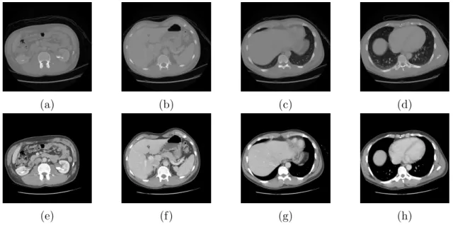
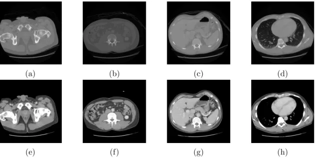
The pixel pitch varied between 0.55 and 0.80 mm, and the slice spacing varied from 1 to 3 mm. Examples can be seen in figure 6.1, which shows consecutive slices with a greater distance between the slices, where the difference in anatomical structures is very noticeable, and figure 6.2, which shows consecutive slices with a smaller distance between the slices, where the differences in anatomical structures structures are more subtle. The dataset used for training is the MICCAI 2007 grand challenge training set (MICCAI-Training), which consists of 10 volume images with corresponding terrain.
Programming Environment
Overview of Liver Segmentation Framework
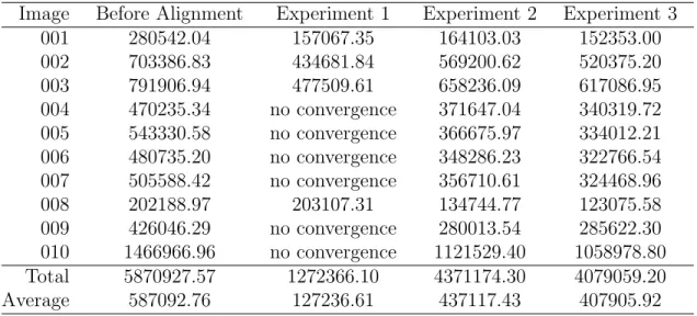
Results of Slice Alignment
Experimental Setup
Evaluation
Results and Discussion
As can be seen from the obtained results, the MSD of the volume obtained by experiment 2 is significantly smaller than that volume before settling. Convergence is faster than in Experiment 1 because slices are aligned with neighboring slices in both directions, ie. the results obtained in experiment 3 are compared with those obtained by Collins et al [23] and Fischer et al [35].
Results of Region of Interest Detection
Experimental Setup
Evaluation
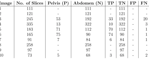
The number of slices per CT volume varies from scan to scan, and so does the number of slices in each class per scan. After the slices are sorted by model, precision, recall, and precision are calculated. Once the slices of all CT scans are evaluated, average scores are calculated and serve as the final scores for the models.
Results and Discussion
The post-training results are shown in Table 6.6 and Table 6.7 for the pelvic plaque detection model and Table 6.8 and Table 6.9 for the breast plaque detection model. For the breast plaque detection model, the achieved accuracy is 0.95, the recall is 1.00, and the accuracy is 0.52. For the breast plaque detection model, the achieved accuracy is 0.97, the recall is 0.86, and the accuracy is 0.92.
Results of Liver Location and Segmentation
Experimental Setup
For the breast disc detection models, this research achieved 0.95 and 0.97 using sparse and deep network models, respectively, whereas AlexNet achieved 0.56 and GoogLeNet achieved 0.58. For the pelvic incision detection models, this research achieved 0.98 and 0.99 using sparse and deep network models, respectively, whereas AlexNet achieved 0.56 and GoogLeNet achieved 0.58. AlexNet and GoogLeNet were pretrained for natural image classification, which may affect its performance in medical image classification.
Evaluation
The segmentation volume is compared to the ground truth volume and the overlap error is calculated in percentage. The segmentation volume is compared to the ground truth volume and the relative volume difference is calculated in percentage. The maximum symmetric surface distance is calculated between the segmentation volume and the ground truth volume in millimeters.
Results and Discussion
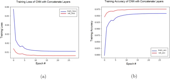
The post-training results are shown in Table 6.20 for a convolutional network model without chained layers. The post-training results are shown in Table 6.21 for a convolutional network model with chained layers. The final results of the framework using CNN with connected layers in the network model are compared with those of related work.
Conclusion
It will also look at what future work can be done to improve the presented framework for liver segmentation described in this thesis.
Conclusion
Summary
- Contributions
Since the liver occurs in the abdomen, the 2D slices containing the pelvis and breast are detected using two CNNs. This is due to the ability of CNNs to learn where the liver is located and segment liver tissue. Finally, experiments were performed to test the effect of the detection method for the region of interest combined with the location of the liver and segmentation with concatenated layers.
Limitations and Future Work
From these results, it is clear that using region of interest detection implementing deep learning techniques improves the accuracy of the entire liver segmentation method. 3D liver segmentation in preoperative CT images using a level-sets active surface method. 31st Annual International Conference of the IEEE EMBS, 8 2009. Automatic liver segmentation method based on maximum a posterior probability estimation and level set method.