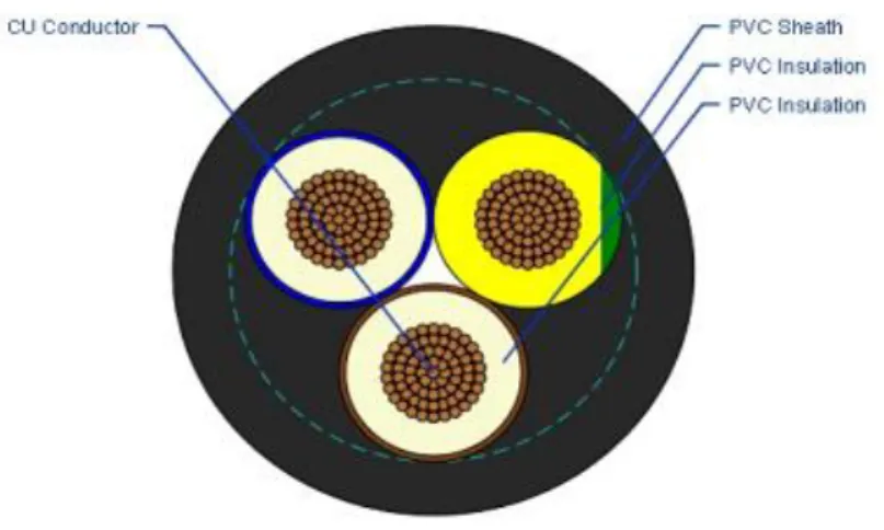
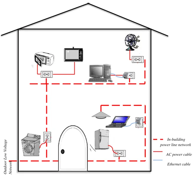
Consistent with its original purpose, the low-voltage line network within a typical in-building structure, as in Figure 1.1, is optimized for the transmission of high voltages at low frequencies, as opposed to data transmission that requires the transmission of low voltage at high frequencies. Therefore, there is an ongoing research into the characterization of the power line as a means of communication.
Research Objectives
In the initial stages of work, most researchers used empirical models to study the behavior of this channel. Accurate measurements are required in the investigation of each channel parameter and their subsequent modeling.
Methodological Approach
A significant contribution to this research is evident in [11] [13] and [15] and all factors contributing to the characterization of the power line channel are studied separately therein. Therefore, once the relationships between the variations of these are obtained, any given network can be sufficiently modeled.
Significance of the Study
Thesis Organization
The accuracy of the transmission line communication channel model largely depends on the primary parameters and the algorithm [11]. Therefore, in this chapter we examine the characteristics of the channel in terms of the primary parameters of the power cables and how they hinder the passage of the signal, to the factors that dictate the behavior of the transmission line channel, that is, the different channel parameters taking into account the time, frequency and location version of the PLC channel.
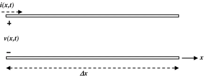
Transmission Line Theory
Primary Transmission Line Parameters
An evaluation of symmetrical three-wire indoor cables for high-frequency signaling, which qualifies the assumption of the two-wire transmission model, is given in [21]. The conductivity per unit length is mainly determined by the dielectric losses of the insulating material between the live and neutral wires.
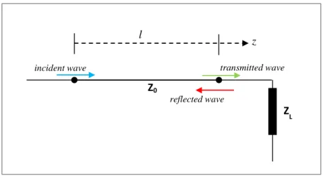
Transmission Line Wave Propagation
Representation by matrices
The ABCD matrix gives the relationship between the input current and voltage and the output current and voltage of the two-port network.
- The Characteristic Impedance
- Impedance at a termination load
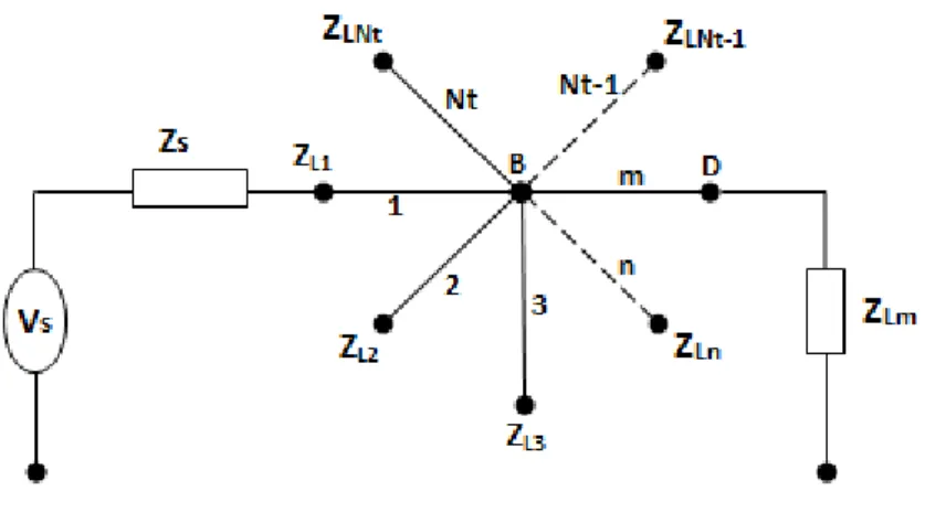
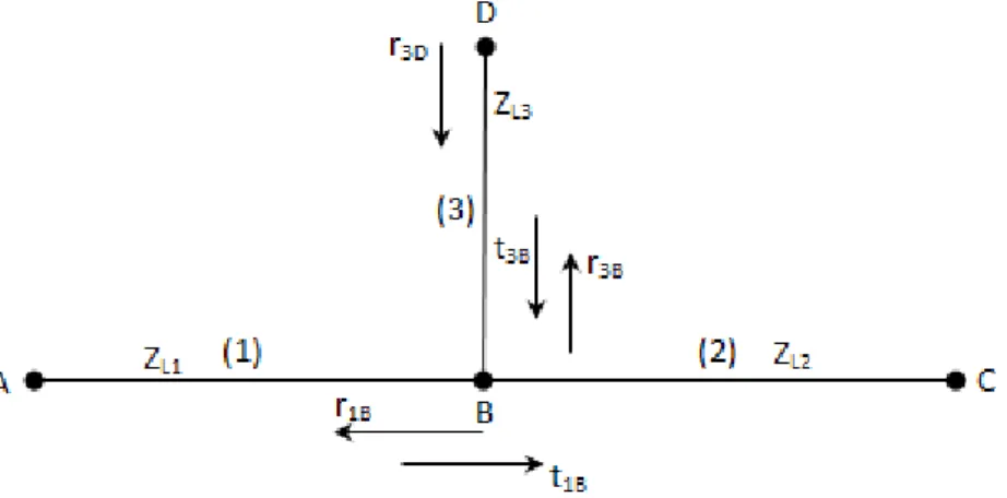
- Impedance at a node
- Input Impedance
- Noise
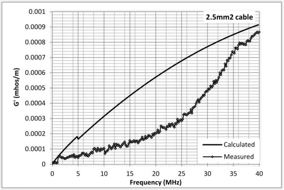
G is mainly influenced by the dissipation factor of the insulating material, which indicates dielectric losses. This is because it depends on the temperature, frequency and composition of the insulating material.
Chapter Summary
Colored background noise, which is mostly generated by low intensity noise sources and not of the nature of those included above. For these models, essentially the two factors that determine the reliability and accuracy of the model are the modeling algorithms and the model parameters. The transfer function parameters are extracted from actual measurements of the given PLC channel or network.
However, the characterization is significantly affected if the values of some parameters are not known. In the following sections of the chapter, a number of models derived from the two modeling approaches are examined.
Top-Down PLC channel modelling .1 Echo Model
Multipath Model
Each path i, representing the product of the reflection and transmission coefficients along the path, has the weighting factor gi. From the complex transfer function measurements of the channel, the parameters of equation (3.5) are obtained. The complex weighting factor of the ide path, which is a combination of the reflection and transmission coefficients of the related path.
For a given number of roads, an estimate of the road damping, weighting and delay factor is determined. The intrinsic line parameters (the characteristic impedance and propagation constant) are derived before the calculation of the transfer function shown in (3.7).
Esmailian et al Model
After calculating the S-parameters for a single branch, the calculation is performed for the entire network by cascading the T-matrices for each branch. Zb = characteristic impedance of the branch cable Zc = characteristic impedance of the cable.
Proposed Model
An evolutionary strategy is used by [12] to determine the optimized component parameters for SRC. When considering measurement results shown by various literature and as shown in the following chapters, the transfer function can be seen as a cascade of the amplitude response of a single SRC, with different resonant frequencies following a certain gradient. Based on measurements in section 5, a correlation was obtained between the notches and the branch characteristics.
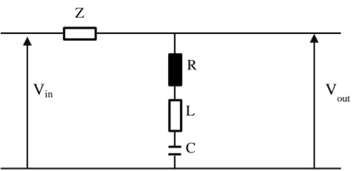
Analyzing the input impedance characteristics around a resonant wavelength λr, circuits in Figure 3.12a and Figure 3.12b behave like a series RLC circuit [53]. We therefore take Figure 3.10 to represent our equivalent circuit for the branch line as in Figure 3.9.
Chapter Summary
After discussing the modeling techniques, algorithms and parameters used to formulate the power line communication channel transfer functions, the calculation of accurate distribution parameters of the cables forming the PLC networks is considered an important aspect in PLC research. The following sections outline the techniques and measurement setups used to obtain the parameters of low voltage cables commonly used in the construction of power networks. The cables used in carrying out measurements were the Cu and Cabtyre flexible PVC cables.
Line Parameter Extraction Technique
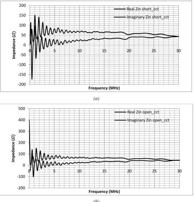
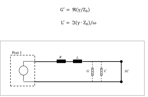
If the terminal is shorted, making ZL equal to zero, (4.1) the input impedance is given by. For each cable, the network analyzer provides an estimate of the reflection coefficient versus the measured frequency, f. The purpose of the measurements is to obtain the unit length values of the distributed elements for our cables, to compare them with theoretical results.
To measure these parameters, we short the end of the cable, effectively establishing a connection through the series elements R' and L', as illustrated in Figure 4.2a, and then measure the complex input impedance. To measure these parameters, we open the end of the cable, effectively establishing a connection through the shunt elements G and C, as illustrated in Figure 4.2b, and then measure the complex input impedance.
Line Parameter Measurements Results
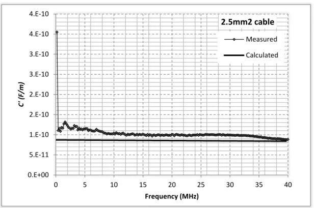
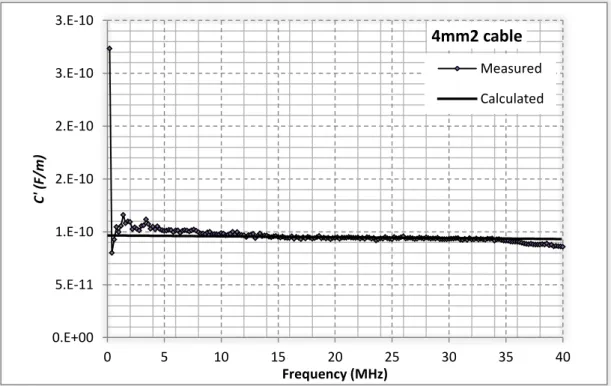
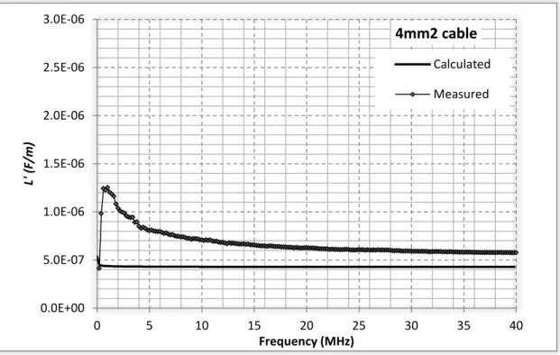
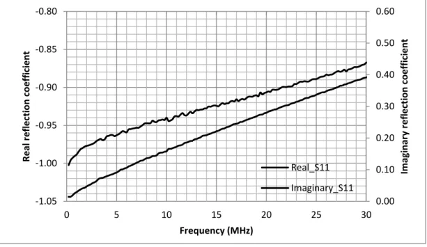
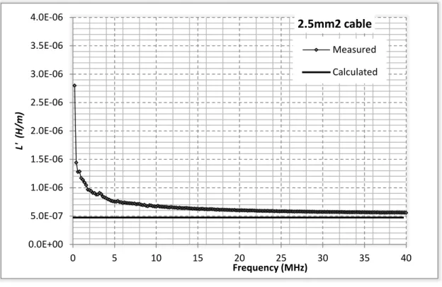
The length of the cable is comparable to the wavelength within the frequency range, and the peaks are due to the resonance of the cable at particular frequencies. Taken directly from the vector network analyzer, for the 3x2.5mm2 PVC cable, the normalized S11 complex parameters for short-circuit and open-circuit cable ends are shown in Figures 4.4a and 4.4b, respectively. Figures 4.6a and 4.6b show the inductance per unit length for 4mm2 and 2.5mm2 three-core cables compared to the theoretical model calculation as given in (2.6).
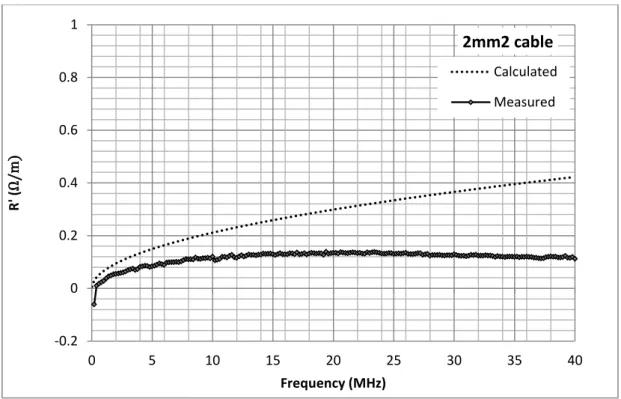
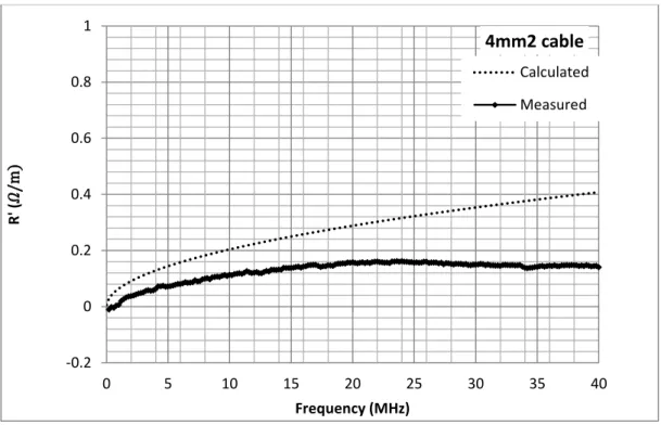
Figures 4.7a and 4.7b show the resistance per unit length for the 2.5 mm2 and 4 mm2 cabtyre three-core cables compared to the theoretical model calculation given in (2.5). Figures 4.8a and 4.8b show the conductance per unit length for the 2.5 mm2 and 4 mm2 cabtyre three-core cables compared to the theoretical model calculation shown in.
The root mean square error (RMSE) between the measured and calculated characteristic impedance values for the 3x2.5mm2 cable is 2.809 and for the 3x4mm2 3.58. However, deviations are noted regarding the resistance and conductivity, which depend on the properties of the dielectric material. This shows that the characteristic impedance mainly depends on the distributed inductance and capacitance parameters of the cable.
However, the composition of PVC varies depending on the manufacturer, so the results in both cases differ.
Propagation velocity
The Attenuation Constant Analysis
Chapter Summary
In Chapter Three, various top-down and bottom-up modeling techniques and their theoretical basis were discussed. Subsequently, in Chapter Four, a precise approximation of the line parameters was determined, which in turn are used to determine the PLC channel constants, the characteristic impedance Z0 and the propagation constant γ. The test setup design, extraction techniques, and channel frequency response measurement results for different configurations are discussed in the following subsections.
Channel Frequency Response Extraction Technique .1 Coupling Method and Circuit
The network analyzer has an input impedance of 50𝛺, the value of the selected capacitor is 10nF. The capacitance of the cable, if not offset, will produce a notch at the resulting resonant frequency within the band of interest. To measure the transfer function of the different networks and topologies, a setup illustrated in Figure 5.4 was used.
All measurements were performed using the Rohde & Shwarz ZVL Network Analyzer. As opposed to turning off all power supply and connecting the analyzer directly, this setup is done to best replicate the actual characteristics of the PLC channel.
Channel Frequency Response Measurement Results
This is due to the cable length being rated in multiples of the relative quarter wavelength. The use of S parameters for characterizing power lines is discussed in Section 3 of Chapter 2. Shown in Figure 5.7a and 5.7b are |S11| and |S22| parameters for different network configurations of a branch, respectively.
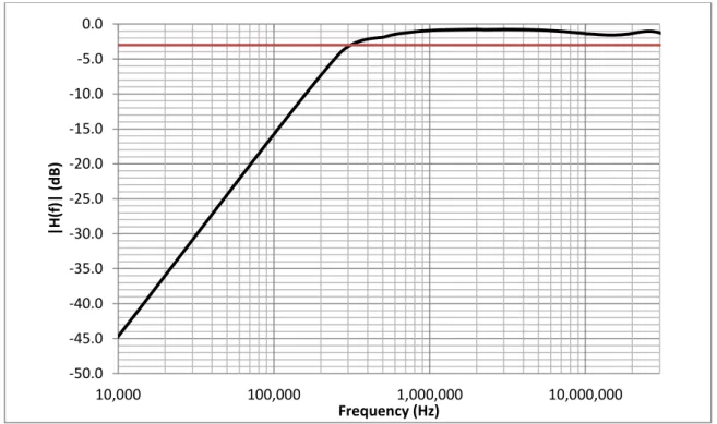
Typical characteristics of channel transfer functions are points at various points and low-pass filter characteristics. The 2-branch network transfer functions also have deep peaks at selected frequencies as well as a low-pass filter characteristic.
Comparison of models to measurements .1 One branch network
Two branch network
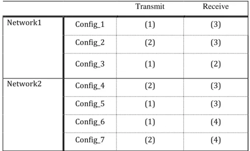
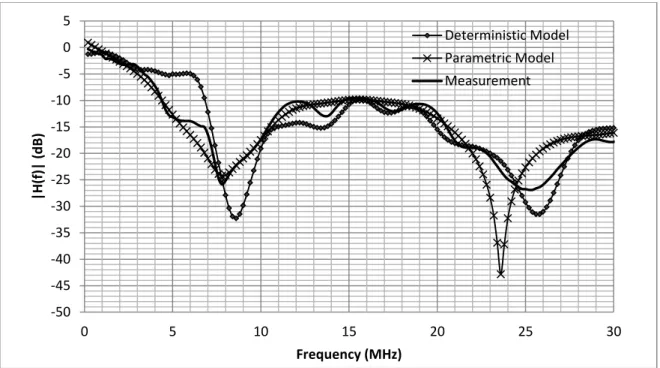
For config_6, the channel frequency response for a two-branch network is compared with a deterministic model [11] and a parametric model with [34], as shown in Figures 5.16 and 5.17.
Comparison to Proposed Series Resonant Circuit Model
The effect of Network Topology Variation .1 Cascading two networks
Based on the ability of the deterministic model in [11] to replicate the transfer function of the PLC channel given the channel characteristics, analysis of the variation in network topology is also performed using this model and the transfer function for the different branch lengths shown in Figure 5.24. We consider the electrical length of the branch expressed in units of the wavelength λ, related to the propagation speed and the signal frequency f by equation (2.1). Given the first notch of the open circuit terminated branch termination, solving for d will give a value of 15.5m.
The extreme cases for the branch load impedance, i.e. short-circuited and open-circuited branch termination are considered and measurements taken are shown in Figure 5.26. The analysis is also done using the deterministic model by [11] and the transfer function for open-circuit, short-circuited and matched terminations plotted in Figure 5.27. The corresponding load branching gives a transfer function without deep notches and close to that of the regression fit of the transfer functions that determines the average path loss.
Chapter Summary
A correlation of the channel response characteristics to some different topologies of the transmission line communication channel is formed. Andreou, “Electrical parameters of low-voltage power distribution cables used for communication over power lines,” IEEE Transactions On Power Delivery, Vol. Dostert, “A multipath signal propagation model for a transmission line channel in the high frequency range,” Proceedings of the International Symposium.
Yamada, "An estimation method for the transfer function of indoor power conduits for Japanese houses," in Proc. Banwell, “A New Approach to Accurate Modeling of the Indoor Power Line Channel—Part II: Transfer Function and Channel Properties,” IEEE Trans.