Application of Deep Convolutional Neural Network in Breast Cancer Prediction Using Digital Mammograms

(1)

Application of Deep Convolutional Neural Network in Breast Cancer Prediction Using Digital Mammograms

by

Rafsan Al Mamun 18301033 Gazi Abu Rafin

21241072 Adnan Alam

21241071 MD. Al Imran Sefat

21241076

A thesis submitted to the Department of Computer Science and Engineering in partial fulfillment of the requirements for the degree of

B.Sc. in Computer Science/Computer Science and Engineering

Department of Computer Science and Engineering Brac University

January 2022

(2)

Declaration

It is hereby declared that

1. The thesis submitted is our own original work while completing degree at Brac University.

2. The thesis does not contain material previously published or written by a third party, except where this is appropriately cited through full and accurate referencing.

3. The thesis does not contain material which has been accepted, or submitted, for any other degree or diploma at a university or other institution.

4. We have acknowledged all main sources of help.

Student’s Full Name & Signature:

Rafsan Al Mamun 18301033

Gazi Abu Rafin 21241072

Adnan Alam 21241071

MD. Al Imran Sefat 21241076

(3)

Approval

The thesis titled “Application of Deep Convolutional Neural Network in Breast Cancer Prediction Using Digital Mammograms” submitted by

1. Rafsan Al Mamun (18301033) 2. Gazi Abu Rafin (21241072) 3. Adnan Alam (21241071)

4. MD. Al Imran Sefat (21241076)

Of Fall 2021 has been accepted as satisfactory in partial fulfilment of the requirement for the degree of B.Sc. in Computer Science and B.Sc. in Computer Science and Engineering on January 18, 2022.

Examining Committee:

Supervisor:

(Member)

Faisal Bin Ashraf Lecturer

Co-Supervisor:

(Member)

Moin Mostakim Lecturer

Program Coordinator:

(Member)

Md. Golam Rabiul Alam Associate Professor

(4)

Head of Department:

(Chair)

Ms. Sadia Hamid Kazi Chairperson

(5)

Abstract

Cancer, a diagnosis so dreaded and scary, that its fear alone can strike even the strongest of souls. The disease is often thought of as untreatable and unbearably painful, with usually, no cure available. Among all the cancers, breast cancer is the second most deadliest , especially among women. What decides the patients’ fate is the early diagnosis of the cancer, facilitating subsequent clinical management.

Mammography plays a vital role in the screening of breast cancers as it can detect any breast masses or calcifications early. However, the extremely dense breast tissues pose difficulty in the detection of cancer mass, thus, encouraging the use of machine learning (ML) techniques and artificial neural networks (ANN) to assist radiologists in faster cancer diagnosis. This paper explores the MIAS database, containing 332 digital mammograms from women, which were augmented and preprocessed, and fed into a custom and different pre-trained convolutional neural network (CNN) models, with the aim of differentiating healthy tissues from cancerous ones with high accuracy. Although the pre-trained CNN models produced splendid results, the custom CNN model came out on top, achieving test accuracy, AUC, precision, recall and F1 scores of 0.9362, 0.9407, 0.9200, 0.8025 and 0.8572 respectively while having minimal to no overfitting. The paper, along with proposing a new custom CNN model for better breast cancer classification using raw mammograms, focuses on the significance of computer-aided detection (CAD) models overall in the early diagnosis of breast cancer. While a diagnosis of breast cancer may still leave patients dreaded, we believe our research can be a symbol of hope for all.

Keywords: breast cancer, malignant, benign, mammogram, CAD model, convolutional neural network, convolution layer, overfitting, MIAS database, accuracy, precision, recall, F1, ROC curve, AUC

(6)

Dedication

We dedicate this research project to all the women who have lost their lives to breast cancer, to all those mothers who have glued together families selflessly without much caring about their health, to all those young ladies who are shut down from raising concerns about sensitive issues, to all those girls who feel hesitant to talk about their physical and mental troubles with others, to all those males who think only their female counterparts should be worried about breast cancer and not them, and finally, to every person in the world competing in a constant rat race to emerge at the top, not realising that it is their health that should be of utmost priority to them.

(7)

Acknowledgement

First and foremost, we would like to show our gratitude to Allah the Almighty, who has given us guidance and His blessings for which we could finish our research work on time with utmost diligence.

Secondly, we would like to extend our deep appreciation to our supervisor, Mr.

Faisal Bin Ashraf and co-supervisor, Mr. Moin Mostakim who have shown us the way throughout the research and helped us finalise it.

Last, but not the least, we thank our parents who have supported us and believed in us for the whole of our lives, and without whom we would have never even reached the stage we are in right now.

(8)

List of Figures

1.1 Dividing Breast Cancer Cell [31] . . . 2

1.2 Region-Specific Incidence and Mortality Rates for Female Breast Can- cer, 2020 [57] . . . 2

1.3 General Overview of the Proposed Solution . . . 5

2.1 Overview of the Basic Structure of a CNN [44] . . . 7

2.2 Convolutional Operation With Zero Padding [44] . . . 8

2.3 Common Activation Functions Used in CNN [44] . . . 9

2.4 Operation of a Max Pooling Layer [44] . . . 10

2.5 Division of Dataset for Training a Model [44] . . . 12

2.6 Fixed Feature Extraction of Transfer Learning [44] . . . 14

3.1 Comparison of AUC Between ANN and Radiologists as Calculated in [15] . . . 17

3.2 Comparison of AUC for Unaided Vs Aided Mammogram Analysis [51] 18 3.3 Mammogram Sample With Labelled Data From [35] . . . 19

3.4 ROC Curve of the Model Used in [42] With AUC . . . 20

3.5 Confusion Matrix Analysis for (a) ResNet50 and (b) VGG16 [52] . . . 22

3.6 ROC Curves of the Models Trained on (a) DDSM and (b) INbreast [52] . . . 22

4.1 Sample Mammograms from MIAS Dataset [4] . . . 26

4.2 Sample Mammogram Before and After Augmentation . . . 28

5.1 Dataset Segmentation for Training and Testing Models . . . 29

5.2 Architecture of ResNet50 . . . 31

5.3 Architecture of MobileNetV3-Small [50] . . . 32

5.4 Architecture of VGG19 [47] . . . 33

5.5 Architecture of Custom CNN Model . . . 34

5.6 Sample ROC Curve . . . 36

6.1 ROC-AUC of the Models . . . 39

6.2 Training Vs Validation Metrics of the Models . . . 40

(11)

List of Tables

2.1 Common Last Layer Activation Functions for Particular Tasks 56 . . 10

3.1 Accuracy of Different Models used in [43] . . . 15

3.2 Accuracy Comparison of Methods from Papers Cited in [28] . . . 16

3.3 Accuracy of Different Models Used in [39] . . . 17

3.4 Comparison of Results Between the Models Used in [35] . . . 20

4.1 Variables Used and Their Instances From the MIAS Database [4] . . 25

4.2 Distribution of the Study Population in MIAS Dataset [4] . . . 25

6.1 Test Accuracy, Loss and Training Times of the Models . . . 38

6.2 Average Precision, Recall and F₁ Scores of the Models . . . 42

(12)

Nomenclature

Adam Adaptive Moment Estimation AI Artificial Intelligence

ANN Artificial Neural Network

AUC Area Under Curve

BI-RAD Breast Imaging - Reporting and Data System CAD Computer Aided Detection

CC Craniocaudal

CLAHE Contrast Limited Adaptive Histogram Equalisation CNN Convolutional Neural Network

CPU Central Processing Unit

CV Cross Validation

DCGAN Deep Convolutional Generative Adversarial Network DDSM Digital Database for Screening Mammography

DMR Research Data Base

DNN Deep Neural Network

FFDM Full-field digital mammography

FN False Negative

FP False Positive

FPR False Positive Rate GPU Graphics Processing Unit

HIPAA Health Insurance Portability and Accountability Act of 1996 IEEE Institute of Electrical and Electronics Engineers

kNN k-Nearest Neighbour

LDA Linear Discriminant Analysis

(13)

LVQ Learning Vector Quantisation

MIAS Mammographic Image Analysis Society

ML Machine Learning

MLO Mediolateral Oblique

MQSA Mammography Quality Standards Act

NB Na¨ıve Bayes

OpenCV Open Source Computer Vision

PEIPA Pilot European Image Processing Archive ReLU Rectified Linear Unit

ResNet Residual Neural Network

RF Random Forest

RGB Red Green Blue

RIAC Rule Induction through Approximate Classification RMSprop Root Mean Square Propagation

ROC Receiver Operating Characteristic ROI Region(s) of Interest

SGD Stochastic Gradient Descent SVM Support Vector Machine

TN True Negative

TP True Positive

TPR True Positive Rate VGG Visual Geometry Group

WDBC Wisconsin Diagnosis Breast Cancer WHO World Health Organisation

(14)

Chapter 1 Introduction

1.1 What Is Cancer?

Cancer is one of the leading causes of death among the world population keeping the life expectancy prisoned to its barriers throughout the globe [56]. According to the research approved by the World Health Organisation (WHO), in 2020 alone, it claimed an estimated 10 million lives [55], [58].

In human body, cell division is a natural process where normal cells divide to replace the dead cells or replicates for growth. However, when cancer develops, this orderly process breaks down, resulting in the cells to become abnormal: old or damaged cells survive when they should die, and new cells form when they are not needed.

These extra cells can divide without stopping and may form growths called tumours, which are divided into two types: malignant and benign. Malignant are the ones that spread and invade the other cells and organs, otherwise known as cancerous, whereas benign ones grow in its place into a large mass [31].

1.1.1 Breast Cancer and its Severity

Breast cancer is one such type of cancer. It occurs when the cell tissues of the breast become abnormal and uncontrollably divides. These abnormal cells form large lump of tissues, consequently becoming a tumour [16], [36]. Figure 1.1 shows a dividing breast cancer cell [31].

Breast cancer is considered as one of the most frequent non-skin cancers that develops in women, such that it is estimated that 1 out of every 8 women will develop it in their lifetime, making it one of the main causes behind women death [12], [36].

According to WHO, in 2020, breast cancer had the highest number of new cases (2.26 million), making it the most common type of cancer, surpassing lung cancer.

It also reported 685,000 deaths, with ratio of 1 in 3 breast cancer patients who succumb to death [58]. Figure 1.2 below depicts the region specific incidence and mortality age-standardised rates for female breast cancer in 2020 [57].

(15)

Figure 1.1: Dividing Breast Cancer Cell [31]

Figure 1.2: Region-Specific Incidence and Mortality Rates for Female Breast Cancer, 2020 [57]

1.1.2 Problems of Diagnosing Breast Cancer

Even though breast cancer is the most frequent malignancy in women worldwide, it is curable in ∼70–80% of patients with early- stage, non- metastatic disease or phase, but is difficult to cure if it reaches distant organ metastasis [46]. However, as we have observed the ratio of deaths to new found cases, it boils down to the fact on how it was not diagnosed sooner when it was still in its early-stage. This again

(16)

reflects certain social aspects, such as in the developing countries where the educa- tion regarding this matter is neither that high nor is it encouraged, especially since it is a sensitive matter and most women are not comfortable to talk or think about it.

However, the biggest problem associated with misidentification of breast cancer is the inability to detect malignant breast tumours from mammography. The detection of masses by the mammography and making a classification and proper image out of it is very challenging particularly because of the varying size and density of female breasts. Radiologists, almost all the time, have issues with it because only 3% of the required information to determine the tumour and its type from normal tissue is being recovered from a mammogram [36]. This is a vital obstacle because, as stated earlier, breast cancer can be treated if it is detected early.

1.1.3 ML and its Use in Breast Cancer Diagnosis

Because of the difficulty of identifying breast cancer from mammograms by radiologists, it is necessary to develop and employ newer techniques to effectively and efficiently discover them. One such technique is using ML to make an artificial intelligence (AI) model that can detect such subtle features and apply its vast knowledge that it accumulated from training through a large data set to find the cancer cells effectively [36]. These can even detect the differences in various micro-calcification deposits or clusters of calcium in soft breast tissues- and masses which are very similar and are hard to distinguish, which usually form from the early onset of breast cancer [12].

A particular ML technique, known as CNN, uses a group of multiple neurones in various layers, taking on image type data, to find necessary patterns in them. It is designed to automatically and adaptively learn spatial hierarchies of features through back-propagation by using multiple building blocks, such as convolution layers, pooling layers, and fully connected layers [44]. These convolutional layers create feature maps that record a region of image which is ultimately sent out for nonlinear processing.

Therefore if a CNN model is trained with these raw mammograms, it should be able to detect the various patterns in the abnormality of a cancerous tissue compared to that of the normal tissue with higher accuracy in regards to other current techniques.

Hopefully, these will give doctors a better chance to diagnose and treat patients with breast cancer from earlier onset.

1.2 Problem Statement

In this paper, the research focus is to classify a patient as cancerous (breast cancer) or healthy, Res(t) which takes on the values 1 (patient has breast cancer) and 0 (the patient is healthy) based on, the probability that a patient has breast cancer, P(C), given a digital mammogram, M of the patient and threshold, t, where t is the cutoff value of the probability beyond which the mammogram will be classified as cancerous. This is more formally defined by:

(17)

Res(t) =

(1 ; P(C|M ∩t)≥t

0 ; P(C|M ∩t)< t ; 0.00≤t≤1.00 (1.1)

Cancer is the second major cause of death globally, accounting for about 1 in 6 deaths [57]. Among all the types of cancer, breast cancer is the most prevalent with about 7.8 million alive women with breast cancer diagnosis at the end of 2020.

Women with breast cancer loses the most disability-adjusted life years than with any other types [58]. The risk of developing breast cancer by women is so critical, especially towards the later life, that even if all the potential risk factors, including avoidance of alcohol and tobacco, avoidance of using hormones, weight control etc, it would only reduce the risk of the onset of breast cancer by a mere 30% [58]. Hence, according to medical practitioners around the world, early detection is the most effective measure of minimising the risks from breast cancer, with mammography being the best cancer screening test at the moment [45].

However, interpreting mammograms pose great difficulties for the radiologists, as most breast cancers can go undetected. This is mainly because women have breasts of varying densities, and the fact that breast tumours are too small to be detected in the early stages. Typically women with dense breasts are more likely to have false-negative results, giving them a false sense of security [48]. Thus, there is a rising need for CAD models to help radiologists have a better diagnosis.

The literature review revealed the mass use of different ML models to differentiate between cancerous and healthy breasts with good accuracy, by using clinical data extracted from the mammograms by radiologists. Albeit other papers have utilised digital mammograms in detecting malignant tumours with the help of CNN, they used pre-identified regions-of-interest (ROI) [33], including lesions, to only target a part of the images. However, in order to build a better CAD model to try help the radiologists identify malignant tumours in breast mammography, it is adamant that the model makes use of the raw digital images of the the mammogram during the identification process, instead of specific ROI and being overly-dependent on radiologists. A model with such capabilities would help detect many cancerous tissues, that could have otherwise gone unnoticed by radiologists.

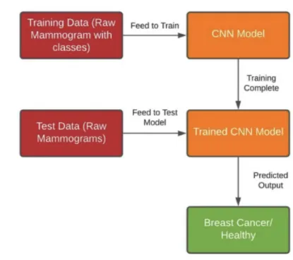
In this paper, the main focus is to accurately identify breast cancer using CNN by utilising raw mammograms, without any prior intervention by radiologists or other medical personnels. Figure 1.3 gives an overview of the solution that is being proposed in this paper. The aim is to show the capability of AI in breast cancer detection, after being trained with a large enough dataset, that would have otherwise gone unnoticed and postulate the significance of better CAD models to help radiologists with early detection of breast cancer, possibly saving thousands of lives in the process.

(18)

Figure 1.3: General Overview of the Proposed Solution

1.3 Research Objectives

In order to build a CNN capable of accurately detecting breast cancer among patients, it is necessary to set a standard procedure for attaining it. This would not only allow to assess the model based on a particular standard, but would also remove biases from the evaluation of the performance of the model.

In this research paper, digital mammograms from the MIAS database [4] have been extracted and augmented, to be fed into different CNN models in order to identify malignant breast tissues without the use of any pre-identified ROI as inputs. Apart from using already-existing pre-trained CNN models, another CNN model that was tailor-made for solving this particular problem would also be used to compare the results. For the purpose of discrimination, the models would be evaluated based on their accuracy of predicting healthy and cancerous breast tissues, precision, recall, F₁ score and the area-under-curve (AUC) of their receiver operating characteristic (ROC) curve plotted using their respective 1-specificity and sensitivity at different threshold values.

The CNN model that has the best above-mentioned metrics, along with lower loss and minimal overfitting, would be proposed for use in detecting breast cancer. The intention is to assert the significance of CNN-based CAD model using raw digital mammograms in the early and better diagnosis of breast cancer.

1.4 Paper Orientation

This chapter mainly introduces the readers to breast cancer, and provides a brief discussion of the research’s problem statement and objectives. The remainder of the

(19)

paper is organised as follows: Chapter 2provides an overview into the background knowledge for this paper, introduces the concept of CNN and justifies the use of CNN for this research. Chapter 3contains the literature review of some past published researches on the use of ML and deep learning in classifying healthy and cancerous tissues in breast cancer patients. Chapter 4 focuses on the dataset, its analysis and preprocessing for being able to be used in the research. Chapter 5introduces the models that were used in this research, with their results being analysed in Chapter 6. Chapter 7 provides a brief discussion about the probable factors that helped the custom CNN achieve supremacy, some limitations of the research and their proposed improvements. Chapter 8 summarises the whole research and concludes the paper. Finally, there is a Bibliography at the end that lists out all the sites and journals that were referred to in this paper.

(20)

Chapter 2 Background

2.1 Convolutional Neural Network

Convolutional Neural Network (CNN) is a neural network model which falls under deep learning which processes data by using a grid pattern, i.e. images, developed by analysing the organisation of the visual cortex of animals [1], [2] which helps it to find differences in low to high level feature patterns.

A CNN has three components: convolution layer, pooling layer and fully connected layers. The task of the convolution and pooling layer is to extract features and can be run multiple times to extract additional features. The extracted features are passed on to the fully connected layers so that it can be mapped on to the output for functions like classification. The more layers the CNN has the more progressively complex the outputs become.

The model is trained for optimisation using different optimisation algorithms like backpropagation, gradient descent etc so that the outputs produced are more con- sistent with the “ground truth” labels. Figure 2.1 gives an overview of the basic structure of a CNN [44].

Figure 2.1: Overview of the Basic Structure of a CNN [44]

(21)

2.2 Building Blocks of CNN Architecture

A typical CNN is made up of several convolutional and pooling layers, connected to fully connected layers. A typical architecture usually consists of repetitions of several convolution layers and pooling layers, followed by one or more fully connected layers.

The step where input data are transformed into output is called forward propagation.

2.2.1 Convolution Layer

The convolution layer plays a vital role in extraction of features by using linear and non-linear mathematical operations such as convolution operation and activation function.

Convolution is the mathematical combination of two functions to produce a third function. It merges two sets of information. In CNN, it is used by applying a small array of numbers known as a kernel or filter on the input data known as tensors.

The elements of the kernel and tensor take part in an element-wise product specific to the individual location of the tensor and summed which results in the creation of a feature map which consists of outputs having unique positions in the output tensor. Moreover, multiple different kernels are applied to the input tensor to extract different features from the datasets.

The convolution operation has two main arguments and they are size and number of kernels. Most common kernel size is 3×3 while 5×5 and 7×7 are also seen. Conven- tionally, convolutional operations do not allow the centre of the kernel to overlap the outermost element of the input tensor meaning the loss of data in the feature map, which can be countered by employing a technique called zero padding. Figure 2.2 shows a convolution operation with zero padding [44].

Figure 2.2: Convolutional Operation With Zero Padding [44]

(22)

A stride is the distance between two successive kernel positions and is commonly 1.

However, a larger one is sometimes used to downsample the feature maps.

Weight sharing refers to the kernels being shared between image positions is an important factor of the convolutional operation. This allows for the local features detected by one kernel to be used as variables by other kernels so no time is wasted detecting local features again. Spatial hierarchies of feature patterns can be learned by downsampling and using a pooling operation, which results in a larger feature map. Moreover, the efficiency of the model can be increased by reducing the number of parameters that are required.

2.2.2 Non-linear Activation Function

The feature map produced from the convolution layer is later passed on to a nonlinear activation function. The most common activation function is the rectified linear unit (ReLU). Figure 2.3 below shows some common activation functions used in the inner layers of a CNN [44].

Figure 2.3: Common Activation Functions Used in CNN [44]

2.2.3 Pooling Layer and Max Pooling

The pooling layer is used for downsampling the feature map’s size in order to introduce a translation invariance which detects small shifts and distortions, and helps to decrease the number of parameters learned during training.

Max pooling is the favoured pooling operation where the feature map is split into groups of patches and the highest value is chosen from each patch and the rest get discarded as shown in Figure 2.4 [44]. The filter size 2×2 with a stride of 2 is the most popular max pooling. This downsamples the feature map by a factor of 2.

(23)

Figure 2.4: Operation of a Max Pooling Layer [44]

2.2.4 Fully Connected Layers

The outputs of the convolutional and pooling layers are connected to one or more fully connected layers in which every input is connected to every output by a learnable weight. Once the features have been extracted by the convolution layer and been downsampled by the pooling layer, they are passed on to fully connected layers which produce the final outputs like probabilities for classification etc. The number of classes determine the number of output nodes in the final fully connected layer.

Each layer is followed by a nonlinear function, such as ReLU, as described above.

2.2.5 Last Layer Activation Function

The activation function used in the last layer is different to the functions used in the other layers and the function used is dependent on the task. Table 2.1 below shows the last layer activation function that are typically used for some particular tasks [44].

Task Last Layer Activation Function

Binary Classification Sigmoid

Multiclass Single-class Classification Softmax Multiclass Multi-class Classification Sigmoid Regression to Continuous Values Identity

Table 2.1: Common Last Layer Activation Functions for Particular Tasks 56

2.3 Training a Network

A network is trained to find a combination of unique kernels in the convolution layer and weights in the fully connected layers that produce outputs with minimum difference from the labeled dataset used. Backpropagation is the main algorithm used for training neural networks with hidden layers which uses the loss function

(24)

2.3.1 Loss Function

Loss function is a function that calculates the difference between the actual output and the output from the network by using forward propagation, and this is labeled as the cost. The most popular loss function for multiclass classification is crossentropy and for regression to continuous value, mean squared error is used. The one used in this paper is the binary cross-entropy.

2.3.2 Gradient Descent

Gradient descent is an optimisation algorithm whose main function is to minimise the loss by regularly updating the learnable parameters like kernels and weights in the network. However, the algorithm that will be used in this paper is known as Adaptive Moment Estimation (Adam), which is more of an improvement upon the general gradient descent algorithm.

2.3.3 Adam Optimiser

Adam is an adaptive learning rate optimisation algorithm and is often referred to as a combination of two optimisation algorithms which are Root Mean Square Prop- agation (RMSprop) and Stochastic Gradient Descent (SGD) with momentum [23].

This is said because, to scale the learning rate, it squares the gradients like RMSprop and uses the moving average of the gradient instead of the gradient like SGD with momentum. Being an adaptive learning rate method means different parameters result in different learning rates. Adam uses adaptive moment estimation, and so to adapt the learning rates of each weight, it uses the estimates of the first and second moments of the gradient. Adam also keeps an exponentially decaying average of past gradients. These are done by using the following formulae [23]:

m(t) =ˆ m(t)

1−β1(t) (2.1)

v(t) =ˆ v(t)

1−β₂(t) (2.2)

where,m(t) = first moment, v(t) = second moment, β1 and β2 = hyperparameter, t = batch number.

The typical values forβ1 and β2 are 0.9 and 0.999 respectively. In order to update the weight, Adam uses the following formula:

θ_t+1 =θ_t− η qv(t) +ˆ ε

m(t)ˆ (2.3)

where,θ = weight, η = learning rate ,ε = zero-avoidance parameter = 10e⁻⁸.

(25)

2.4 Data and Ground Truth Labels

In any machine learning methods or deep learning, datasets and ground truth labels are the most important content. In fact the success of any such method and models are dependent on its dataset and ground truth label. Therefore, it is most necessary to carefully select the datasets and ground truth labels, but then again, obtaining such high quality ones is both expensive and time consuming [44]. As for medical images, there are multiple good quality sources readily available. However, to be used for a specific topic or specific function, the model needs data sets with particular ground truth labels and hence, special care needs to be taken.

Usually datasets are of 3 categories: a training, validation and test set. As the name suggests, the training set is used to train the network, where loss values are calculated via forward propagation and learnable parameters are updated back into the network via backpropagation. Validation set is used for fine-tuning the hyperparameters and performing model selection during the whole training process. At the very end, the final model or network is run through the test set and its final performance after all those tuning using training and evaluation datasets is evaluated (see Figure 2.5 [44]). It is notable that evaluation and test sets are kept different. This is particular because the training model’s hyperparameters are fine-tuned according to the performance it showed while using the evaluation set.

Figure 2.5: Division of Dataset for Training a Model [44]

2.5 Overfitting

Overfitting is the phenomenon when a model learns the statistical regularities specific to the training set, in other words it learns the unnecessary information or noise particular to the dataset instead of the signal, hence performing poorly on the new dataset. Overfitting has always been a challenge and thus, the test set is

(26)

used to evaluate the performance of the model. Regular checkup to recognise the overfitting to the training data by monitoring the loss and accuracy to the training and validation sets is usually done [44].

Although there are solutions to avoid these in practice, the best solution to avoid overfitting of course is to have more training data. However, given such is not always available, there are other ways such as regularisation with dropout, weight decay, data augmentation etc [44].

Dropout is a regularisation technique, where randomly selected activations are set to 0 during the training, so that the model becomes less sensitive to specific weights in the network [18]. Weight decay or L2 regularisation penalises the model’s weights so that it takes only small values. Batch normalisation is a type of supplemental layer, which standardises the input values of the following layer for each mini batch adaptively, thus, reducing overfitting. It has the effect of stabilising the learning process and dramatically reducing the number of training epochs required to train a deep network. Data augmentation, on the other hand, is a process where the training data is modified through random transformations, such as flipping, translation, cropping, rotating, random erasing etc, so that the model sees different input while training [37], [44].

2.6 Transfer Learning

Although large datasets are highly desired in training a model, such datasets are hard to find. One way to mitigate this problem is to use transfer learning, as it trains the network model on a large dataset, like ImageNet, then reuses the pre-trained model for the topic of interest. The assumption that is made is features learned on a large dataset can be shared among seemingly disparate datasets [44]. This ability to shift the learned generic features from datasets is what gives deep learning the advantages to make itself useful in various domain tasks with small datasets. Some examples of such models are AlexNet, VGG, ResNet etc.

While there are many ways to use the pre-trained network, this paper will focus on fixed feature extraction. A fixed feature extraction method is a process to remove fully connected layers from a network pre-trained on a large database, while maintaining the remaining network, which consists of a series of convolution and pooling layers, referred to as the convolutional base, as a fixed feature extractor (see Figure 2.6 [44]). The fixed feature extractor can further be topped off with fully connected layers in CNN resulting in training limited to the added classifier on a given dataset of interest [44].

(27)

Figure 2.6: Fixed Feature Extraction of Transfer Learning [44]

2.7 Why Use CNN for This Research?

Over the years, CNNs have developed much rapidly, thanks to its ability to accurately conduct difficult classification functions in images that would have otherwise required abstract concepts. What gives CNN an edge compared to its old com- petitors is its ability to detect important features in a dataset without the need for any human supervision, making it the go to model for a lot of industrial systems.

As stated before, the core concept of CNN is that it uses different convolutions and filters to produce invariant features that are passed on to the next layer, where more new filters and convolutions are applied to extract further features, until it gives a final output.

However, the key feature of CNN is that it works well on image data, as the several convolution layers derive benefit from the fact that an interesting pattern can occur anywhere in an image, in contiguous blocks of pixels, allowing it to learn useful features from raw data without manual image processing. Since the purpose of this research is to predict breast cancer from raw image data with complex features, CNN is more than capable of standing up to the task, producing better predictions than any other models. Hence, CNN was chosen to be used for this research.

(28)

Chapter 3

Literature Review

As stated earlier, to be able to better facilitate subsequent medical treatments, it is really necessary to be able to detect malignant breast tissues. Breast cancer is usually detected after the conductance of a special type of X-ray, called a mammography, which is later scrutinised by radiologists for a better diagnosis. However, it has been revealed that in about 1 in 5 breast cancers get undetected by radiologists after screening [48]. Hence, it is understood that CAD techniques, especially ML, could aid radiologists to have a better interpretation of the patients. Thus, a number of past papers that have tried to incorporate such techniques have been reviewed to find the scope of further research and have been summarised below.

3.1 Research Using Clinical Data

Most papers have used clinical data gathered from mammograms as a means of detecting breast cancer. One such paper [43] used the commonly used ML techniques, namely Random Forest (RF), k-Nearest Neighbour (kNN) and Na¨ıve Bayes (NB).

For reference, the author has cited different other papers: Detection using Relevance Vector Machine [32] yielded results with an accuracy of 97%, using the Wisconsin Diagnosis Breast Cancer (WDBC) dataset [3]; Mamdani Fuzzy inference model for training was used in one study in conjunction with Linear Discriminant Analysis for feature selection and acquired an accuracy of 93% [26]. The paper [43] utilised the WDBC dataset [3], consisting of 569 instances attributed mainly by diagnosis, mean radius, mean texture, and mean area of the ROI, split it into 10 different chunks using the 10-fold cross validation (CV) method, and fed them into said ML models.

The accuracy of the models can be found in Table 3.1 [43]. Although the author produced great accuracy exceeding 94% in breast cancer identification, the dataset was too small to be used to train non-parametric models like NB, increasing chance of overfitting.

Method RF kNN NB

Accuracy (%) 94.74 95.90 94.47

Table 3.1: Accuracy of Different Models used in [43]

(29)

Similar to the one above, another paper [28] has also utilised the WDBC dataset [3], albeit an updated one with 699 instances. The study proposed the use of a new NB technique, called a weighted NB, to classify breast tissues as malignant or benign. The dataset used had 9 different clinical features, namely clump thickness, uniformity of cell size, uniformity of cell shape, marginal adhesion, single epithelial cell, bare nuclei, bland chromatin, normal nucleoli and mitosis, for each of the patients. The author used a similar technique as [43] to validate the model, known as the 5-fold CV. However, since the author used a weighted NB, using weights to control the attributes in a posterior probability contribution meant that changes should be done to the original NB equations to properly represent them, bringing a big disadvantage of assigning crisp classes to the training data [13]. The author further used a heuristic search algorithm to calculate the weights to be used. After training and testing the model, the author achieved an average accuracy of 98.54%.

Table 3.2 depicts a comparison of the author’s model with other papers the author has cited [28]. Even though the author was able to manipulate the NB classifier to achieve greater result than others, while doing so, the paper introduced a heuristic search algorithm that is computationally expensive on which the model is dependent to obtain the weights, along with a bias that cannot provide generalised result when used on other datasets.

Study Method Accuracy (%)

Hamilton et al. [5] RIAC 94.99 Ster and Dobnikar [6] LDA 96.80 Bennett and Blue [7] SVM 97.20 Setiono [9] Neuro-rule 98.10 Goodman et al. [10] Big-LVQ 96.80

This study [28] W-NB 98.54

Table 3.2: Accuracy Comparison of Methods from Papers Cited in [28]

It seems like the WDBC dataset [3] is a popular choice among researchers trying to discriminate breast cancer patients from healthy ones using ML techniques. An- other recent paper [39] utilised the same dataset for use in NB and kNN classifiers for breast cancer classification. The authors of this paper split the dataset into training and testing set in the ratio of 60:40 respectively, before feeding it to a standard kNN model with k=3. For the NB, the authors calculated the mean and standard devia- tion of each feature for each category (malignant and benign), which were then used to calculate the probability for each prediction the model made. However, the model had a poorer accuracy than kNN as seen in Table 3.3 [39]. This research, apart from suffering from small dataset, might have also suffered from under-training since only 60% of the dataset has been used solely for training, thus reaching a lower accuracy than [28] despite resorting to a similar model, albeit a simpler one.

(30)

Method kNN NB Accuracy (%) 97.51 96.19

Table 3.3: Accuracy of Different Models Used in [39]

The use of clinical features extracted from mammograms has not only been used in typical ML models, but also in ANNs, in order to achieve even better results. A paper from the year 2010 [15], was one such paper that made use of a feed-forward ANN, with 36 discrete input variables, split using the 10-fold CV method, and a hidden layer with 1000 nodes. The paper not focused on discriminating the benign cells from the malignant cells, but also on stratifying patients into high and low risk groups. The paper worked with over 60000 mammography findings matched with the Wisconsin State Cancer Reporting System, consisting of a 5-level BI-RADS assessment [11]. The ANN, trained with early stopping method to avoid overfitting, achieved a significantly higher mean AUC (0.965) compared with that of radiologists (0.939; p¡0.001)) calculated from their respective ROC curves as seen in Figure 3.1 [15]. The authors evaluated the accuracy of their model’s risk prediction by using the Hosmer-Lemeshow goodness-of-fit test [21], which showed a high calibration.

The results demonstrated that this model may have the potential to help the radiologists in discriminating between benign and malignant breast tissues. The difference of the AUC between the ANN and the radiologist may look small (0.026) but this difference is significant both statistically and clinically as the model identified 44 more cancers and decreased the number of false positive by 3941 when compared with the radiologists. However, the one flaw in this research was the fact that the authors depicted a BI-RAD score of 0 as positive, whereas in reality, the score 0 means unsure, hence, causing some inaccuracies in their result.

Figure 3.1: Comparison of AUC Between ANN and Radiologists as Calculated in [15]

(31)

3.2 Research Using Digital Mammograms

The papers cited in the previous section mainly centred their attempts of building CAD models to help in the accurate detection of breast cancer among patients using primarily the clinical data extracted from the mammograms and the patients.

However, another way of detecting breast cancer is by analysing the mammographic images using a CNN without the need of other clinical inputs. This is more likely to ensure a better CAD model that do not rely on radiologists’ interpretation, but rather try to find the specific patterns in the images by itself.

One such paper [51] that incorporated the idea of CNN for breast cancer classification, compared the breast cancer detection performance of the radiologists reading the mammograms unaided versus supported AI systems. This was an an enriched retrospective, fully crossed, multi-reader, multi-case, HIPAA-compliant study, which used digital mammographic examinations from 240 women. The mammograms were later interpreted by 14 Mammography Quality Standards Act (MQSA) - qualified radiologists, with and without AI support. The system used deep CNN, features classifiers and image analysis algorithms to depict calcifications and soft-tissue lesion in two separate modules, which were then combined to determine suspicious region findings. These regions were later given values between 1 and 100 which represented the level of suspicion that breast cancer was present (with 100 indicating the highest suspicion). Figure 3.2 shows the difference between the AUC of the ROC curves for the two reading conditions, compared by using mixed-models analysis of variance and generalised linear models for multiple repeated measurements [51]. The paper could have been an excellent case for showing the power of AI in the detection of breast cancer and its superiority over radiologists. Unfortunately, however, the results were not much promising as the AUC difference between the radiologists’

investigation with and without AI support was a mere 0.02, with p=0.002 (the difference is not significant). Hence, it calls for better CAD models that can analyse raw images to classify breast cancer patients.

Figure 3.2: Comparison of AUC for Unaided Vs Aided Mammogram Analysis [51]

(32)

Another paper that has studied the detection of breast cancer from mammograms by utilising a CNN but with much better results than [51] was the paper from [35]. However, before diving into building the models arbitrarily, the author has into previous works in order to grasp the different types of breast cancer and how they are classified with the use of multiple kinds of ANN that specialise in image classification. Firstly, the CNN tutorial on TensorFlow was used in order to test the functionalities of the features it offers [24]. Secondly, for image classification, a model from [19] which was the ImageNet Classification with deep CNN was looked at and the preprocessing techniques present were used as references in [35]’s work.

The dataset used in the paper was from the mini-MIAS, containing 322 grayscale mammograms with labelled data, describing the type of cancer, properties of the background tissue, class of abnormality and the coordinates of the centre of abnormality. The authors further used image transformations techniques in order to augment the dataset. A random mammogram sample from this dataset has been shown in Figure 3.3 [35]. Unlike other researches, the authors used three different versions of CNN to assess their results: one was the CovNet model from Kaggle [34], second CNN model was developed following the TensorFlow tutorial [24] that takes the whole image as input with labelled data, and the third used a 48x48 input matrix, convolution layer with kernel size 5x5 filter with ReLU activation, pooling layer with max pool size 2x2 filter and a stride value of 2, learning rate with 0.003, and training step with 20,000 samples. Their results have been tabulated in Table 3.4 [35], which shows the third version surpassing the other two with 82.71% accuracy.

Although the model could have been improved by removing the labelled data from the images, it still shows the capabilities of AI to help the doctors in this field to correctly identify breast cancer, if present, in the patient faster.

Figure 3.3: Mammogram Sample With Labelled Data From [35]

(33)

Version Version 1 Version 2 Version 3 Sensitivity (%) 35.32 54.32 82.68 Specificity (%) 35.43 54.36 82.73

Accuracy (%) 38.45 54.35 82.71

Table 3.4: Comparison of Results Between the Models Used in [35]

When searching for more studies which used neural networks for classification of mammograms, two further studies of interest were found that met the search criteria. The first one [20] used an ANN and the second one [22] used a wavelet neural network to identify breast cancer. However, both of these methods have a lot of parameters (∼3 million) when compared to a normal CNN (∼600) as they were made for making general decisions.

Next, there was one paper [42] that was of particular interest because of its use of an unorthodox methods of detecting breast cancer from images. This study first explored infrared imaging, that assumes that there is always an increase in thermal activity in the precancerous tissues and the areas surrounding developing breast cancer. The study used the Research Data Base (DMR) database containing frontal thermogram images, including breasts of various shapes, from 67 women.

The thermograms went through image pre-processing to mark the ROIs and remove the unwanted regions like arms, neck etc. They were then fed into an AI model built using a deep neural network (DNN) together with a Support Vector Machine (SVM) model as classifier. The SVM is only consulted with if the DNN is incapable of classifying the images with great confidence. The model which is presented in this paper takes advantage of two main factors. First, a DNN (pre-trained Inception V3 model [30], [40]) which is modified at the last fully connected layer in such a way as to obtain a powerful binary classification which can tell if a cell is healthy or cancer infected. Secondly, a well known classifier (SVM) is coupled to that and is involved only in the case of uncertainty in the output of the DNN. The results of this study is presented in Figure 3.4 [42] that shows an AUC of 1.00 calculated from its ROC curve. Even though the study has shown a perfect accuracy of detecting breast cancer, such models should be dealt with extreme caution as, ironically, such accurate models could also be a result of overfitting, which could be particularly true in this case because of the extremely small dataset used in the study.

Figure 3.4: ROC Curve of the Model Used in [42] With AUC

(34)

Finally, the best paper in this category, in terms of the sophistication of the model used and the accuracy attained, [52] had a goal of detecting breast cancer from screening mammograms by using a deep learning algorithm, trained by an “end-to- end” approach, allowing the datasets to be either complete clinical annotations or only the labeled cancer region in the image. Many studies before it applied deep learning models, but these models were used to classify annotated lesions because ROI in a mammogram is too small when compared to a full-field digital mammography (FFDM). Some studies were also found that used unannotated FFDM datasets to train neural networks, but the results were inconclusive [38], [41].

The dataset used in this study [52] were taken from the DDSM database which included a total of 2478 mammography images taken from 1249 women. The mammograms consisted of standard views such as craniocaudal (CC) and mediolateral oblique (MLO) and these views were used as separate images. The images consisted of annotations for the ROIs, the type of cancer and whether it was a mass or calcification. The sampling of image patches from the ROIs and background regions resulted in a lot of images which were later split into two datasets: S1 and S10. S1 consisted of a mix of image patches which focused on the centre of ROIs and random background patches from each of the images, while S10 had 10 patches randomly selected from the regions surrounding the ROI coupled with background patches to paint a big picture of the ROI. These patches were further classified as background, malignant mass, benign mass, malignant calcification and benign calcification. This dataset was used in the pre-training of the classifier. Another dataset from the INbreast database was also used in this study. This dataset had 410 mammograms with CC and MLO views from 115 patients. The mammograms had radiologists’ BI-RADS assessment which were: 1-no findings, 2-benign, 3-probably benign, 4-suspicious, 5-highly suggestive of malignancy and 6-biopsy-proven cancer.

The images with BI-RADS 3 were excluded and BI-RADS 1 and 2 were labeled as negative and 4, 5 and 6 as positive. This dataset was used to train the whole image classifier.

This study made the model in such a way that it needed a fully annotated lesion dataset only during pre-training for the initialisation of the weight parameters of the model, and then labeled images without ROI annotations could be used for the rest of the training. This is beneficial as large databases of annotated lesions are hard to come by. For pre-training usually a two step method is used which is made up of classification of the annotated ROIs by a classifier which generates a grid of probabilistic outputs and these outputs are summarised to find out the classification of the outputs to their respective classes. The author suggested a new method which combines both of these steps in order to optimise it. This is done by using the input patches found in the images and putting them directly into a CNN classifier instead of a conventional classifier. The output from the CNN is a grid of probabilistic outputs of the classes instead of it being classified into single classes.

Two CNN structures were used in this study: the VGG network [29] and the residual network (ResNet) [27], specifically a 16-layer VGG network (VGG16) and a 50-layer ResNet (ResNet50) respectively. The results of using the VGG16 and ResNet50 on the DDSM dataset are shown as a confusion matrix in Figure 3.5 [52], that tell both

(35)

networks performed well overall but struggled with correctly identifying malignant classifications followed by correctly identifying malignant mass.

Figure 3.5: Confusion Matrix Analysis for (a) ResNet50 and (b) VGG16 [52]

Lastly, two hybrid networks have been created by first adding the best performing VGG blocks as top layer (two VGG block of (256)×1 and (128)×1) and the ResNet50 as bottom layers and vice versa (two blocks of (512-512-1024)×2). Moreover, to further efficiently train the networks, augmentation prediction was used which meant that the model trained on each image was flipped vertically and horizontally resulting in four images and the average AUC of the four images was used. After all this training, four models were identified as top performing and they were (patch classifier-top layer): ResNet-ResNet, VGG-VGG, ResNet-VGG and VGG-ResNet.

This marked the end of the training of the model using annotated lesions. Next, the best models were trained on the INbreast dataset. The annotations on this dataset were ignored as the authors wanted to focus on the performance of the whole image classifiers on unannotated lesions and the transferability. The ROC graphs of these networks trained on the DDSM and INbreast datasets can be seen from Figure 3.6 [52]. The INbreast dataset produced a mean AUC of 0.95 (higher than DDSM) from all the four models. Moreover, using an ensemble of all the models resulted in an AUC of 0.98 and scored 86.7% and 96.1% in sensitivity and specificity respectively.

Figure 3.6: ROC Curves of the Models Trained on (a) DDSM and (b) INbreast [52]

(36)

However, trying to achieve such high accuracy comes with its prices. To begin with, it is found that to efficiently train the network during pre-training to provide op- timum results, the network requires a large number of patches or large patches in general. Using large patches means that the computational cost also linearly in- creases. Furthermore, large patches require more GPU memory in order to process them properly. In addition, the whole image classifier was trained on the INbreast dataset which was labeled based on the BI-RADS provided by the radiologist, which has a chance of being wrong. The classifier being trained on it means it will incorporate a bias instead of finding new unknown characteristics in the images. Even so, nonetheless, this study shows the power of using end-to-end training deep learning models to produce highly accurate results in depicting breast cancer from mammograms, which can then easily be transferred to other datasets with little effort.

3.3 Major Findings and Scope of Research

After an exhaustive search through a corpus of past papers that had made use of ML techniques and deep learning for the classification of breast cancer, there were three main findings that would set the base for this paper:

1. Most researchers usually opt for clinical data extracted from mammograms as opposed to using the whole image to train the ML models for breast cancer identification. These assessments, especially the BI-RADS scores are subject to human-error, leading to inaccuracies in the results of the models.

2. Although some papers have tried to incorporate the idea of using images, most had used specific ROI as targets for the models to analyse, instead of trying to explore the whole mammogram for favourable features. This again causes the models to be over-reliant on radiologists’ observation and speculation of a specific region that needs to be targeted.

3. Even if some papers have been able to achieve high accuracy and AUC from their models for breast cancer detection, most of them had used a relatively small dataset than that is required to effectively train the models. As a result, these models might not be proficient enough to generalise over unseen data.

The study in this paper is to be carried away in such a way as to minimise the effects of the above mentioned observations. The study intends to incorporate unannotated digital mammograms taken from the MIAS database [4] classified into normal, benign and malignant breast samples, which would be augmented to increase the size of the dataset for a better CAD model. CNN models are intended to be used to extract features from the dataset, in order to find patterns to aid in the detection of breast cancer patients.

Although a paper [35] tried to use raw images without specific ROIs in CNN, it failed to achieve better accuracy mainly due to the model’s simplicity. The paper, that utilised the MIAS dataset, would be used as the comparison base for this research, with the intention to build a CNN model sophisticated enough to be able to handle the problem at hand, and ultimately help doctors detect breast cancers in patients early and with better confidence.

(37)

Chapter 4 The Dataset

4.1 Data Collection

All the mammograms from the database of the Mammographic Image Analysis Society (MIAS) [4], an organisation of UK research groups who are particularly interested in the understanding of mammograms, have been included in the dataset used in this paper for a retrospective evaluation. The films, compiled in the year 1994, were taken from the UK National Breast Screening Programme and had been digitised to 50 micron pixel edge with a Joyce-Loebl microdensitometer. The dataset was then further reduced to 200 micron pixel edge and had been clipped and/or padded to make all the images of size 1024x1024 pixels, hence the name, mini-MIAS.

The final dataset is available via the Pilot European Image Processing Archive (PEIPA) at the University of Essex [4].

4.2 Data Analysis

The mini-MIAS database comprised of 328 digital raw mammograms belonging to 161 patients (image of left and right breasts of each individual). 6 of the mammograms were duplicates and so, have been removed to reduce the dataset to 322 samples. For each of the mammograms, the database contained the reference number, breast density, the abnormality present, severity of the abnormality, the x and y coordinates of the centre of abnormality, and the approximate radius of a circle enclosing the abnormality as can be seen in Table 4.1 [4].

When calcifications were present in the image, the coordinates and the radii apply to a cluster instead of individual calcification, with the bottom-left corner taken to be origin. Moreover, in some cases, the calcifications were distributed throughout the image rather than concentrating in a single site, for which the coordinates and radii are inaccurate and so, have been omitted.

The mammograms were prospectively analysed and interpreted by experienced radiologists who had between 1-35 years of experience in breast imaging. Their in- terpretations have been considered as the “ground-truth” values for the purpose of this research.

(38)

Variables Instances

MIAS Reference Number 6-digit reference number

Breast Density -Fatty (F)

-Fatty-glandular (G) -Dense-glandular (D) Abnormality Present -Calcification (CALC)

-Well-defined/circumscribed masses (CIRC) -Spiculated masses (SPIC)

-Ill-defined masses (MISC)

-Architectural distortion (ARCH) -Asymmetry (ASYM)

-Normal (NORM) Severity of Abnormality -Benign (B)

-Malignant (M)

Coordinates of Centre of Abnormality x, y image-coordinates Radius of Area of Abnormality Radius (in pixels)

Table 4.1: Variables Used and Their Instances From the MIAS Database [4]

In order to properly analyse the dataset, the study population have been distributed based on certain criteria as can be found in Table 4.2 [4]. As can be seen, almost two-thirds (64%) of the total study population had normal breast tissues, with only 16% having malignant breast tumours and the rest having benign. Figure 4.1 shows random sample mammograms of patients with normal, benign and malignant breast tissues [4].

Study Population Normal (%) Benign (%) Malignant (%) Total (%)

No. of mammograms 207(64) 65(20) 50(16) 322(100)

Breast Density

Fatty 66(20) 22(7) 18(6) 106(33)

Fatty-glandular 65(20) 22(7) 17(5) 104(32)

Dense-glandular 76(24) 21(6) 15(5) 112(35)

Abnormality Present

Calcification - 12(4) 13(4) 25(8)

Well-defined/ - 19(6) 4(1) 23(7)

circumscribed masses

Spiculated masses - 11(3) 8(3) 19(6)

Ill-defined masses - 7(2) 7(2) 14(4)

Architectural distortion - 9(3) 10(3) 9(6)

Asymmetry - 6(2) 9(3) 15(5)

Table 4.2: Distribution of the Study Population in MIAS Dataset [4]

After a careful analysis of the dataset, it can be seen that most of the study population (35%) had dense-glandular breasts. It is worth noting that, people with this density of breasts were least identified as having malignant breast tissues (5%), and most identified as having normal breast tissues (74%). Now, this could either

(39)

Figure 4.1: Sample Mammograms from MIAS Dataset [4]

be a normal phenomenon or it could re-iterate the fact that it is difficult to detect breast cancer in dense breast as stated earlier. Hence, there could be some level of discrepancies in the radiologists’ assessment, but, since the difference is quite small compared to other breast densities, this has been neglected.

Moreover, it could also be seen that most breast tumours were in the form of calcification (8% among total and 22% among patients with tumour) and well- defined/circumscribed masses (7% among total and 20% among patients with tumour), while the least common form of tumour was ill-defined masses (4% among total and 12% among patients with tumour). It should also be noted that, among patients with a malignant tumour, almost 16% had a combination of fatty breast tissue and calcifications, which is the highest.

However, since the purpose of this research is to be able to predict breast cancer from raw digital mammograms, without relying on radiologists’ clinical assessments and ROI, these clinical data have not been used in the models. Rather, only the raw image files and their interpreted labels have been incorporated in them.

4.3 Data Preprocessing for Use in Models

Before the images can be used in the CNN models, they need to be preprocessed in order to ensure that there are no bias or discrepancies in the models’ predictions due to the nature of the data.

4.3.1 Data Segmentation

Since the research being done is to predict if a patient has breast cancer or not, the multiple segmentation of the dataset, i.e. normal, benign and malignant, are not needed to train the models. Hence, the dataset has been divided into 2 categories:

“healthy” (patients having normal and benign breast tissue) and “cancer” (patients having malignant breast tissue). Therefore, the final dataset now had the original 322 images split into a ratio of 272:50 into the 2 categories respectively.

(40)

4.3.2 Data Augmentation

As stated early, one of the key improvements this research would have over others mentioned in the literature review, is to mitigate the disadvantage of working with a small dataset. When a neural network model is given a small-sized dataset to train, that model becomes overfitted, and memorises the data instead of the relationships.

The goal of a model is to generalise patterns from the training data so that it can predict new data which was not available during training. The fewer the samples for training, the more models tend to become an overfitting model. Thus, the images need to be processed and augmented for the total dataset to increase in size. The preprocessing steps were done using the OpenCV [8] and Albumentations [54] library and are as follows (see Figure 4.2):

1. Resize to 224x224 pixels: The images were scaled down proportionally from the original 1024x1024 pixels to 224x224 pixels. This was mainly done to reduce the complexity of working with a large array of pixels, and also because the pre-trained models to be used in this research has an input size of 224x224 pixels.

2. Shift from RGB channel to LAB colour space: In order to apply Con- trast Limited Adaptive Histogram Equalisation (CLAHE), images need to be turned to grayscale from RGB. However, since the input channel of most popular pre-trained models is RGB, the images had to be shifted to the LAB colour space (L, A, B stands for luminescence, red/green coordinates and blue/yellow coordinates respectively), so that CLAHE could be applied to the luminescence channel.

3. Equalised using CLAHE and shifted back to RGB channel: Contrast Limited Adaptive Histogram Equalisation (CLAHE) is a variant of Adaptive Histogram Equalisation which takes care of over-amplification of the contrast, and improves its quality [53]. CLAHE was applied on the images using a clip limit of 5. Later, the images were converted back to the RGB channel to be fed into the models. The resulting images after applying CLAHE were used as the base to apply the later augmentations on.

4. Rotation: The images were rotated anticlockwise by 10 and 20 degrees, to make the changes look subtle.

5. Flip: The images were then flipped both on the vertical and the horizontal axis.

6. Random Tone Curve: This method randomly changes the relationship between bright and dark areas of an image by manipulating its tone curve. This too was applied to ensure colour distortion of images were not an issue when making predictions.

7. Gaussian Noise: Gaussian Noise is a statistical noise having a probability density function equal to normal distribution. This noise was added to introduce some graininess in the images.

(41)

8. Blur: The images were also blurred by using a random-sized kernel, although the blurriness was kept tenuous to ensure minimal distortion of the original images.

After the completion of all the augmentation steps, the dataset, which once had only 322 mammograms, now contained 2898, with a total of 2448 mammograms belonging to the healthy category and the rest 450 to the cancer category.

Figure 4.2: Sample Mammogram Before and After Augmentation

(42)

Chapter 5 The Models

After performing the preprocessing steps mentioned in Chapter 4, the dataset is ready to be fed into CNN models to establish a relationship between the features of the mammograms and the final interpretation. The dataset was further split in 80:20 ratio to be used for training and testing purposes respectively. 10% of the training data (8% of the total dataset) was used for validation while the rest for training the models. This was done using SciKit-Learn’s [17] train test split() method using the parameter “shuffling=True” to ensure a mix of classes in each set of data used. This segmentation of the dataset would also allow to analyse if there is any overfitting of the models or not. Figure 5.1 shows the segmentation of the dataset used for training and testing the models.

Figure 5.1: Dataset Segmentation for Training and Testing Models

5.1 Transfer Learning Models

As stated previously in Section 2.6, transfer learning allows the use of models pre- trained on a large dataset to be used for other classification problems, that make use of relatively smaller datasets. The transfer learning models used for this research

(43)

were trained on the ImageNet dataset [14], an image database that has been organised according to the WordNet hierarchy. Containing more than 14 million images, the database has been significant in advancing deep learning research. The models were implemented through the process of fixed feature extraction, by freezing all the layers to retain their learned weights, while replacing the last fully connected layer to fine tune them for this problem-specific tasks. Several models were tested upon using the TensorFlow library [25], and only the best performing ones were further exploited for better efficiency.

5.1.1 ResNet50

ResNet50 is a type of residual neural network (ResNet) model made up of 50 layers, out of which 48 layers are convolutional layers, 1 MaxPool and 1 AveragePool layer. ResNet is popular as it allowed the use of ultra deep neural networks which contained hundreds or thousands of individual layers with great performance [60].

Simply stacking layers on an existing network produces higher error, which ResNet overcomes by performing identity mappings using shortcut connections that skip one or two layers. Hence, one of the biggest advantage of it was that no additional parameters were added to the model while the computational time remained the same.

The ResNet50 architecture contains the following elements (see Figure 5.2):

1. A convolution with a kernel size of 7x7 and 64 kernels with a stride of 2.

2. A max pooling layer with a stride of 2.

3. Convolution layers with 64 1x1 kernels, 64 3x3 kernels and 256 1x1 kernels.

These layers are then repeated 3 times.

4. Convolution layers with 128 1x1 kernels, 128 3x3 kernels and 512 1x1 kernels.

These are then repeated 4 times.

5. Convolution layers with 256 1x1 kernels, 256 3x3 kernels and 1024 1x1 kernels, which too are repeated for 6 times.

6. Convolution layers with 512 1x1 kernels, 512 3x3 kernels and 2048 1x1 kernels, repeated 3 times.

7. An average pooling layer connected to a fully connected layer containing 1000 nodes, ending with a softmax activation function.

For the purpose of this research, the last fully connected layer was replaced by a fully connected layer (after flattening the previous outputs to a one-dimensional vector) with 512 hidden nodes, ReLU activation and a dropout of 0.5, before finally connecting to an output layer with 1 node and sigmoid activation function. Hence, the model now has more than 51 million trainable and more than 23 million non- trainable parameters. The model was compiled using Adam optimiser (learning- rate=0.001), binary-crossentropy as the loss function and accuracy as the metric.

The model was trained and tested using various configurations, but the best average result was obtained by training the model for 8 epochs with 100 steps per epoch,

(44)

Figure 5.2: Architecture of ResNet50

5.1.2 MobileNetV3-Small

MobileNets are a family of CNNs, developed by Google, for the mobile phone and embedded architectures [49]. They are based on a streamlined architecture which makes use of depth-wise convolutions to build lightweight deep CNNs.