Explainable Artificial Intelligence and Model Calibration for Water Quality Prediction

(1)

Explainable Artificial Intelligence and Model Calibration for Water Quality Prediction

by

Nakayiza Hellen 21166042

A thesis submitted to the Department of Computer Science and Engineering in partial fulfillment of the requirements for the degree of

Master of Science in Computer Science and Engineering

Department of Computer Science and Engineering Brac University

August 2022

(2)

Declaration

It is hereby declared that

1. The thesis submitted is my/our own original work while completing degree at Brac University.

2. The thesis does not contain material previously published or written by a third party, except where this is appropriately cited through full and accurate referencing.

3. The thesis does not contain material which has been accepted, or submitted, for any other degree or diploma at a university or other institution.

4. I have acknowledged all main sources of help.

Name & Signature:

Nakayiza Hellen 21166042

Date

(3)

Approval

The thesis titled “Explainable Artificial Intelligence and Model Calibration for Wa- ter Quality Prediction” submitted by Nakayiza Hellen (21166042) in Summer, 2022 has been accepted as satisfactory in partial fulfillment of the requirement for the degree of Master of Science in Computer Science and Engineering on August 9th , 2022.

Examining Committee:

External Examiner:

(Member)

Dr. Md. Haider Ali Professor

Department of Computer Science and Engineering Dhaka University

E-mail: [email protected] Mobile: +8801711988544

Internal Examiner:

(Member)

Dr. Md. Golam Rabiul Alam Professor

Department of Computer Science and Engineering BRAC University

E-mail: [email protected]

Internal Examiner:

(Member)

Dr. Md. Khalilur Rhaman Professor

(4)

Supervisor:

(Member)

Dr. Md. Ashraful Alam Assistant Professor

Program Coordinator:

(Member)

Dr. Amitabha Chakrabarty Associate Professor

Head of Department:

(Chair)

Sadia Hamid Kazi, PhD Chair and Associate Professor

(5)

Ethics Statement

This thesis was carried out in complete compliance with research ethics, norms and codes of practices set by BRAC University. I have ensured that all the sources have been cited.

As the Author of this thesis, I take full responsibility for any ethics code violations.

(6)

Abstract

Water is a key necessity for survival and sustenance of all living creatures. In the past years, the quality of water has been adversely affected by pollutants and other harmful wastes. This increased water pollution deteriorates water quality, making it unfit for any type of use most especially compromising the safety of drinking water for public health. The ecological safety and human health have continuously lowered due to hazardous pollution factors like chemicals and pathogens. By monitoring the Water Quality data parameters and forecasting them to get early warning, we can manage the quality of the water for different water sources. Numerous innovative technologies are slowly replacing human labor and other state of the art methods in water quality evaluation.Recently, different machine learning and artificial intelligence techniques have been adopted for water quality modeling which has become very beneficial in assessment and management of water resources. However, they suffer many times from high computational complexity, high prediction error and the blackbox nature in which they remain. Another big challenge faced by policy makers and other responsible Public Health Authorities is the lack of a relatively generalizable model for water quality prediction for public consumption with provi- sion of explanations for understanding the most influential water quality parameters.

This work presents an Explainable Artificial Intelligence method, SHAP (SHapley Additive exPlanations) to transparently and explainably assess the most important metrics that these models use in determining water quality based on potability. We also model a robust generalizable calibrated ensemble machine learning model for water quality prediction based on water potability and other water quality metrics from various water quality samples around the world. We then implement Auto- mated Machine Learning with Stacked Ensembling to compare its results with those achieved by the Soft Voting Ensemble Model. The simulated results will provide theoretical support to policy makers and would be of interest to water planners in terms of assessing or maintaining water quality and improving sustainable pollution control, water and ecological management plans of water resources as well as early risk assessment and prevention in water environment in a simple, fast and cost-effective way which will protect the health of the people.

Keywords: Explainable Artificial Intelligence (XAI); Machine Learning (ML); En- semble Learning; Water Quality; Public Health; Model Calibration

(7)

I would like to dedicate this research to my mother and heroine, Ms.

Nakawuka Mary and to everyone that has ever taught me something

(8)

Acknowledgement

This report would not have been possible without the contribution and collaboration of others. My sincere gratitude to Almighty who granted me good health and long life, strength, knowledge and wisdom to put together this research work.

Bearing in mind previously I am using this opportunity to express my deepest gratitude and special thanks to my supervisor Dr. Md. Ashraful Alam who inspite of being extraordinarily busy with his duties, took time out to hear, guide and keep me on the correct path and allowed me to carry out this research at their esteemed Computer Vision and Intelligent Systems (CVIS) Lab. In the same spirit, I thank my Thesis Committee members for all their absolutely invaluable discussions, ideas, feedback and guidance throughout the process.

I am grateful to the Brac University International & Scholarship Office for the Academic Merit Scholarship offered to me throughout the tenure of my postgraduate research. I also gratefully extend my appreciation for the Research Financial support provided by the CSE Department Fund (Budget: B.15.4 item category) at BRACU to present our research work at the Consortium of Universities for Global Health (CUGH 2022) Conference.

Lastly, it is my radiant sentiment to place on record my best regards, deepest sense of gratitude to my beloved family members and friends to whom I am, and always will be indebted. I am not sure how I would have managed if it was not for their constant support and encouragement.

I perceive this opportunity as a big milestone in my career development. I will strive to use gained skills and knowledge in the best possible way, and I will continue to work on their improvement, in order to attain the desired career objectives. I hope to continue cooperation with all of you in the future.

(9)

List of Figures

3.1 Turbidity of water . . . 17

3.2 Water pH . . . 19

3.3 Missing Values . . . 21

3.4 Sulfate Values Distribution . . . 21

3.5 High Level Diagram for the Proposed Water Quality Prediction Ap- proach . . . 24

3.6 Dataset Features with Missing Values . . . 25

3.7 Anomaly Plot for the Dataset . . . 25

3.8 Outlier Distribution . . . 26

3.9 Correlation Matrix . . . 27

3.10 PCA Plot . . . 27

3.11 Feature distribution by Potability class and approved limit . . . 28

3.12 Features and p-value based on T-test . . . 29

3.13 Block diagram of Ensemble Learning . . . 30

3.14 An example scheme of stacking ensemble learning . . . 31

4.1 Random Forest Confusion Matrix . . . 34

4.2 Extra Trees Confusion Matrix . . . 34

4.3 Decision Trees Confusion Matrix . . . 35

4.4 Random Forest ROC Curve . . . 35

4.5 Extra Trees ROC Curve . . . 36

4.6 Decision Trees ROC Curve . . . 36

4.7 Random Forest Decision Boundary . . . 37

4.8 Extra Trees Decision Boundary . . . 37

4.9 Decision Trees Decision Boundary . . . 38

4.10 Random Forest Learning Curve . . . 38

4.11 Extra Trees Learning Curve . . . 39

4.12 Decision Trees Learning Curve . . . 39

4.13 Random Forest Feature Importance Plot . . . 40

4.14 Extra Trees SHAP Feature Importance Plot . . . 40

4.15 Decision Trees Feature Importance Plot . . . 41

4.16 Random Forest SHAP Summary Plot . . . 41

4.17 Extra Trees SHAP Summary Plot . . . 42

4.18 Decision Trees SHAP Summary Plot . . . 42

4.19 Random Forest SHAP Force Plot . . . 43

4.20 Extra Trees SHAP Force Plot . . . 43

4.21 Decision Trees SHAP Force Plot . . . 43

4.22 Partial View of Feature Importance with Partial Dependencies . . . . 44

(12)

4.23 Feature Importance based on Mean Decrease in Impurity . . . 44

4.24 Feature Importance based on Feature Permutation . . . 45

4.25 Feature Importance based on Correlation Coefficients . . . 45

4.26 SHAP explanation for effects of data points (features) on Water Qual- ity Prediction using LGBM . . . 48

4.27 SHAP explanation for effects of data points (features) on Water Qual- ity Prediction using CatBoost . . . 49

4.28 SHAP explanation for effects of data points (features) on Water Qual- ity Prediction using Random Forest . . . 49

4.29 Confusion Matrix for the Soft Voting Classifier . . . 50

4.30 Decision Boundary for the Soft Voting Classifier . . . 51

4.31 ROC Curves for the Soft Voting Classifier . . . 51

4.32 Confusion Matrix for the Calibrated Model . . . 52

(13)

List of Tables

1.1 Research papers for the Research Objectives . . . 3

1.2 Tabular visualization of the Thesis Organization . . . 5

3.1 Dataset Features . . . 16

4.1 Results Table . . . 32

4.2 Model Comparison . . . 47

4.3 Performance Evaluation using tuned parameters . . . 47

4.4 Stacked Ensemble Model Classification Report . . . 50

4.5 Calibrated Model Classification Report . . . 52

(14)

Nomenclature

The next list describes several symbols & abbreviation that will be later used within the body of the document

AI Artificial Intelligence CatBoost Categorical Boosting DL Deep Learning

LGBM Light Gradient Boosting Machine M L Machine Learning

P D Partial Dependence RF Random Forest

SDG Sustainable Development Goal SHAP Shapley Additve exPlanations SV M Support Vector Machine

U N United Nations

W HO World Health Organization W QC Water Quality Classification W QI Water Quality Index

XAI Explainable Artificial Intelligence

(15)

Chapter 1 Introduction

1.1 Background

Seventy percent (70%) of the surface of the earth is water and all living creatures on earth require water to survive [4] [6]. It is an extra ordinarily essential component of the wellbeing of man and the aquaculture business [9]. However, water is often times polluted due to rapid urbanization and industrialization[38] [26] every year deteriorating water quality at an alarming rate as harzadous wastes are discharged into the water bodies. This results into worrying diseases, heavy economic losses and increased infant mortality as the children take contaminated water [56] [5].

The World Health Organization (WHO) reported that half of the world population are going to lack water in 2025 and the United Nations (UN) in its 2018 report mentioned that without taking necessary action, challenges will only increase by 2050 yet by then the global demand for fresh water is predicted to have increased by a third. World Vision (as of April 2021) reported that 1 in 10 people which is equivalent to 785 million people do not have access to clean water yet access to clean water can prevent 9% of global diseases and atleast 6% of global deaths.

Water quality deterioration adversely impacts health, environment and infrastruc- ture or development at national, regional and local levels [29] [17]. Another study according to UN indicated that waterborne diseases cause 1.5 million deaths annu- ally, which is way greater than a combination of deaths caused by crimes, accidents and terrorism. Thus surveillance and management of water quality is necessary in combating the negative effects of water pollution and increasing Water Quality too especially for developing countries. Policy-makers and managers around the world have put in place several Water Quality testing and analysis laboratories [41] [32]

and guidelines have been set based on that [30].

(16)

1.2 Motivation

It is very painful that high costs are incurred in carrying out hydrochemical tests to measure a large number of parameters as well as the long delays faced in obtaining laboratory results [61]. On top of that, the sensors used for testing different water quality parameters are very expensive yet their results are not precise. Fortunately, in the past few years, logistic expenses of water sampling have been cut by applying cost effective methods like Machine Learning and Deep Learning solutions for predictive modeling of water quality for precise results at various system stages before water site access under different stages [44] and improvement of water treatment processes [35]. Researchers have comprehensively deployed predictive models but the problem with all the existing models is that they still remain in the blackbox nature.

The alarming consequences of poor water quality raise the need for an alternative method for surveillance and management of water quality, which is quicker and in- expensive and obtaining a global water quality dataset with various water quality metrics to perform water quality modelling. With this motivation, this research demonstrated the water quality features in machine learning modelling using various exploratory data analytic techniques and deployed SHAP to interpret the water quality predictions of the models by transparently and explainably demonstrating how these machine learning models determine Water Quality based on water potability. We then ensembled the best machine learning models and calibrated the final ensemble model that is robust and generalizable enough to precisely predict water quality for human consumption.

1.3 Research Scopes (Gaps addressed)

Limited work has been done to explainably explore influential features for Water Potability using ML and AI techniques. There is also no work identified to focus on exploring feature Learning and interaction in Water Quality Prediction. Moreover all the existing statistical methods used are not interpretably sufficient. Based on the existing literature, no work has been done to explore water quality prediction in terms of water potability. Lastly, the existing Artificial Intelligence models still remain in the blackbox nature. They are not transparent enough to provide explanations of why and how they came up with their accurate predictions. And besides, many other studies used either few or too many parameters which is not efficient enough in predicting the water quality. Generally, Artificial Intelligence application in the field of Water Quality Evaluation is still an under researched thematic area yet its potential in stopping the adverse effects of poor quality water is very enormous.

(17)

1.4 Research Objectives

(a) To prove the concept of Safe Water Quality Evaluation using Machine Learn- ing with a real-world dataset collected for different water resources.

(b) To improve ML and AI interpretability for Public Health Officers, Policy Mak- ers and other concerned authorities by using Explainable AI in more transparent and insightful means for decision making in regards to Water Quality Management.

(c) To derive and comprehensively illustrate the most important features that require extra attention during Water Quality Evaluation.

(d) To create a new robust and relatively generalizable model that is capable of transparently illustrating feature interaction of the most influential features leading to a precise Public Health decision for Water Quality Evaluation.

The above core research objectives of this thesis were investigated through two scientific international conference papers as illustrated in Table 1.1

Table 1.1: Research papers for the Research Objectives

Paper Short Form Research Contributions Objective(s) Investigated PID1- XAI- for - Safe Water

Evaluation

Explainable AI for Safe Water Evaluation for Public Health in Urban Settings

a, b, c

PID2- XAI and EL - for - Water Quality Prediction

Explainable AI and En- semble Learning for Wa- ter Quality Prediction

a, b, c, d

1.5 Research Contributions

1.5.1 Explainable AI for Safe Water Evaluation for Public Health in Urban Settings (XAI-4-Safe Water Evalua- tion) | Objectives: a, b, c

We proposed Interpretable Machine Learning Models for predicting water quality using ten features. We used interpretable approaches to explain the features contributing to the predicted results for Public Health officers or responsible authorities to understand how the machine learning algorithms came up with the predicted results. Below is the summary of our contributions in this paper:

(18)

1. We analyzed the water quality variables.

2. We modeled and trained various Machine Learning (ML) classifiers to predict water quality in an effort to determine water potability.

3. We evaluated the performance of the trained classifiers.

4. We proposed and deployed SHapley Additive Explanations (SHAP) to interpret the prediction for easy understanding of how the ML models arrived at such conclusions and improve transparency and possibilities of adoption of this technology in Public Health.

1.5.2 Explainable AI and Ensemble Learning for Water Qual- ity Prediction (XAI-4-Safe Water Evaluation) | Objec- tives: a, b, c, d

We developed a robust calibrated ensemble learning model for predicting water quality and tested it on a real dataset for Water Potability [47] with ten features and about 3276 samples. The proposed Model showed a recall and precision of over 90% with respect to the dataset. The results may warrant translation of the study outcomes into full-scale Public Health practice by guiding agencies and governments on management, policy and decision making concerning water resources. Below is the summary of our contributions.

1. We performed exploratory data analysis on the dataset.

2. We modeled and trained various Machine Learning (ML) classifiers to predict water quality in an effort to determine water potability.

3. Based on different parameters, we evaluated performance these ML models and provided explanations for the predictions of the best three models using Shapley Additive Explanations (SHAP).

4. We then modeled a robust ensemble model that can be utilized for effective binary classification prediction of Water Potability based on the inputs.

5. And lastly, we calibrated the final model to make it generalizable for water quality prediction.

(19)

1.6 Thesis Organization

The thesis organization is based on research scope Conceptualization and Objectives as investigated by two scientific research papers coded with Research Paper Short Formats in Table 1.1. The tabular visualization of the thesis organization can be studied in Table 1.2.

Table 1.2: Tabular visualization of the Thesis Organization Chapter 1: Introduction Background

Motivation Research Gaps Research Objectives Research Contributions

Thesis Organization (Thesis Outline) Chapter 2: Existing Works Importance of Water for Public Health

Water Contamination and Pollution Water Quality Evaluation

Existing Artificial Intelligence Approaches to Water Quality Analysis and Prediction

Ensemble Learning

Explainable Artificial Intelligence (XAI) Model Calibration

Chapter 3: Methodology PID1 - XAI - for - Safe Water Evaluation Objective(s): a, b, c

PID2 - XAI and EL - for - Water Quality Prediction

Objective(s): a, b, c, d

Chapter 4: Results and Discussion

Chapter 5: Conclusion Major Observations and Lessons Learned Conclusion derived from the Observations Future Works derived from the Observations

(20)

1.7 Research Orientation

The remaining part of this thesis report has been organized as follows:

Chapter 2 briefly reviews how other researchers used AI-based models to predict, detect and evaluate water Quality

Chapter 3 discusses the components of our proposed model, its design and implementation.

Chapter 4 explores results found from different approaches taken towards Water Quality Evaluation

Chapter 5 synopsizes the whole thesis together with the limitations of the thesis work and suggests future potential derivative work for further research.

(21)

Chapter 2

Existing Works

2.1 Importance of Water for Public Health

From a hygienic view point, water is among the important environmental factors which are a source of life, a guarantee of health and important for the plant world.

Water is a sacred gift of Mother Nature that ensures the existence of every living thing on Earth. Water is one of the most abundant substances in nature, oc- cupying 71% of the earth’s surface, 65% of the human body is water, and is an integral component of human production activity [33].

Proximity and access to water are essential for human culture and urban heritage, as well as for health, well-being, and disease prevention. The well-being and safety of residents, as well as community involvement, are highly associated with water [54].

Water as a universal solvent mixes with nature through the hydrological cycle, and it plays many vital roles in human societies and natural ecosystems. Water flows both through living organisms and in the inorganic environment. Additionally, the users of water are diverse and interconnected in multiple ways. Due to the complexity and multiple pathways of water, the essential role of water can be viewed as: a) clean potable water for drinking and maintaining a good immune system; intake of adequate amounts of such water is surely required, b) clean water for safe food production (Clean water is essential for safe food production and maintenance of hygienic conditions in all the food chain links right from the farm to the customers), c) means of keeping hygiene (body washing, indoor and outdoor cleaning) and d) drug and disinfectant production. Water not only sustains life through its major role in the prevention process of diseases but has also been recognized to its essence in alleviating them. It is therefore important that service providers grow their capabilities for providing good quality water due to the significance of handwashing and satisfactory water supply in disease prevention. With all the explained facets of water use, water undoubtedly has a vital role, whether clean in prevention, or contaminated – representing a potential threat. Thus, special attention should be paid to its good usage and management so as to conquer disease outbreaks as quickly as possible.

(22)

Water has broad-ranging applications with some being life needs while others are economical, agricultural or recreational. Water is one of the key substances with influence on human health. Although it is essential to life, it may be a carrier of chemical substances which influence water’s properties and assimilability of water- contained compounds. The assessment of a health risk related to the consumption of water is an essential, multi-stage process that contributes to any evaluation of health effects caused by potential exposure of humans to chemical substances. The constant global growth and the development of industries have increased the water demand.

More economical water management as well as greater attention to water quality, both locally and globally, are the best ways to counteract the threat of global water scarcity. Educational efforts should be adopted in raising awareness concerning the importance and role of water in the environment. It is also necessary to educate the public about the negative effects of anthropogenic activity and pollution on human health [65].

2.2 Water Contamination and Pollution

Water is very fundamental to life but could also be fatal. Despite legal regulations that exist, water can be contaminated with chemical substances posing a serious health risk[65]. The dynamic nature and easy access of water systems makes them vulnerable to contamination and waste disposal effects [19]. Good water quality ensures a longer lifespan of human beings and aquatic creatures. Water species can tolerate certain limits of pollution but a higher extent can jeopardize their survival.

Natural water bodies like rivers, lakes, and streams exhibit their quality through various parameters of quality standards [15]. Therefore, predicting those quality parameters accurately could help in safeguarding the quality and monitoring of the pollution. It is very essential since these water bodies provide water for drinking, agriculture and aquaculture. Since water quality has been susceptible to various pollutants like return flows from agro-industries, industrial waste, domestic waste, fertilizers and pesticides identified as the biggest contributors to surface water contamination, water quality preservation has become urgent for human and hydrous ecosystem issues. It is important to note that continuous population increase increases the need for water resources too. Unfortunately, humans discharge a lot of non-treated waste and contribute to industrial activities which continuously reduce water quality. The safety of water is also compromised by resultants of natural processes like inputs from air and conditions of the climate [23].

2.3 Water Quality Evaluation

Water pollution makes the water unfit for human consumption and for industrial, agricultural purposes as well [57]. Getting water quality to a level needed for public usage requires that water supplies must be managed properly [13] [6]. Water Quality is usually calculated using certain parameters attained through lab analysis. Mul- tivariate statistical methods like Principal Component Analysis and geo-statistical techniques such as kriging, transitional probability, multivariate interpolation, regression analysis have been used to discover the relationship among the various parameters for water quality.

(23)

Water quality requirements differ based on the suggested purpose of water. As stated in [25], ‘water that is unsuitable for one purpose may be satisfactory for another purpose’. These water quality requirements should be in line with the standards put in place by the concerned government agencies. Generally three standard types exist that is; in-stream, potable water, and wastewater with each type having its own criteria using similar measurement approaches.

2.4 Existing Artificial Intelligence (Machine Learn- ing and Deep Learning) Approaches to Water Quality Analysis and Prediction

Superior robustness was identified as the leading categorical parameter when nonlinear autoregressive neural networks, deep learning algorithms and LSTM were used for prediction of Water Quality Index using a dataset with 7 significant parameters.

LSTM was outperformed by the NARNET model in predicting WQI values based on the R-value and the SVM algorithm achieved better accuracy (97.01%) compared to K-nearest neighbor and Naive Bayes for Water Quality Classification [20].

To predict Total Dissolved Solids of aquifers, adaptive fuzzy inference system (AN- FIS), artificial neural network (ANN) models and support vector machines (SVMs) were used and Principal Component Analysis was used for determining the most influential inputs for prediction of Total Dissolved Solids [21]. These models were trained using moth flam optimization, cat swarm optimization, particle swarm optimization, shark algorithm, grey wolf optimization, and gravitational search algorithm. The hybrid ANFIS-MFO improved the Root Mean Square Error accuracy over the SVM-MFO and ANN-MFO models by 3.8%, and 1.4% respectively. The ANFIS-MFO further enhanced the Root Mean Square Error by approximately 3%

and 7%, as compared to the ANN-MFO and SVM-MFO. The ANFIS-MFO and ANFIS-CSO models showed superior performance compared to other models thus indicating significant implication in their application for other hydrological variables and water resources in general.

A Neuro-Fuzzy Inference System (WDT-ANFIS) based on augmented wavelet denoising technique was proposed. Three techniques or assessment processes were used for evaluating the models with the first depending on partitioning of the neural network connection weights in ascertaining the significance of every network input parameter and the second and third assessment processes ascertaining the most ef- fectual input to construct the models using individual parameters and a combination of parameters, respectively. Two scenarios were presented for these processes. Sce- nario 1 was constructing a prediction model for water quality parameters at every station, while Scenario 2 was developing a prediction model based on the value of the same parameter at the previous station (upstream). Both scenarios were ex- perimented using twelve input parameters. The WDT-ANFIS model significantly improved the prediction accuracy for all water quality parameters and outperformed all other models. Furthermore, the performance of Scenario 2 was more adequate

(24)

compared to that of Scenario 1, with substantial improvement of 0.5% to 5% for all parameters at all stations [12].

A model that utilizes principal component regression was proposed for prediction of water quality. At first, the weighted arithmetic index method was used to calculate WQI and PCA was applied to the dataset to extract the most dominant parameters.

In the next step, to predict the WQI, regression algorithms were applied to the Principal Component Analysis output to predict the Water Quality Index (WQI) and lastly the Gradient Boosting Classifier was used for classification of the water quality status. The principal component regression method achieved 95% prediction accuracy while Gradient Boosting Classifier method achieved 100% classification accuracy [46].

Artificial Neural Network algorithms with early stopping, Ensemble of ANNs and ANNs Bayesian Regularization were used to predict the Water Quality Index using 16 ground water quality parameters. Comparing performance of the algorithms for prediction of Water Quality Index (WQI) indicated that the Bayesian regularization method indicated successful WQI prediction. For the training and testing datasets, the correlation coefficients between the predicted and observed values of the Water Quality Index were 0.77 and 0.94 respectively. Sensitivity analysis was deployed to demonstrate each parameter importance during ANN modeling and Phosphate and Iron (Fe) were the most dominant in WQI prediction.

Auto Deep Learning was compared with the conventional Deep Learning model in predicting water quality. The conventional Deep Learning approach gave a slightly better performance compared to AutoDL for both binary and multiclass water data but adoption of Auto Deep Learning made finding an appropriate Deep Learning model easier and gave better performance minus manual intervention [63].

Effectiveness of eight Artificial Intelligence methods in prediction of water quality in a dry desert environment was studied based on two scenarios and two different input combinations that is; replacement of the classical computational method with modeling approach and lack or unavailability of data in critical cases [48]. The models were evaluated by means of various statistical metrics including mean absolute error (MAE), root mean square error (RMSE), root relative square error (RRSE), relative absolute error (RAE) and correlation coefficient (R). The experimental results showed that TH and TDS were the key influential factors in predicting WQI in the study area. In the first scenario, the MLR model achieved the highest accuracy amongst all models and in the second scenario, the RF model exhibited less error. The results suggested that Random Forest algorithms could be a robust and cost-effective model for enhancement of groundwater quality management plans in such a study area.

(25)

Several supervised Machine Learning–based models were tested in an effort to assess the Water Quality Index and Water Quality Class based on four parameters that is; pH, turbidity, temperature and total dissolved solids. From the experiments, the gradient boosting algorithm performed best with a learning rate of 0.1 and polynomial regression, with a degree of 2, predicted the Water Quality Index most efficiently with a Mean Absolute Error of 1.9642 and 2.7273, respectively [6].

A deep learning model that utilizes Long-Short Term Memory (LSTM) algorithm was proposed for IoT systems. The model was forecasting Water Quality indicators that is; salinity, temperature, pH, and dissolved oxygen necessary to monitor Water Quality (WQ) for aquaculture and fisheries. The results obtained after experiment- ing showed that the proposed model is fit for real-world application. Additionally, monitoring of the indicators and generation of early warnings from the system could help farmers in managing water quality [34].

The proposed approach utilized two hidden layer types that is; the LSTM layer and a fully connected dense layer while the ambient temperature prediction task was formulated as a time series regression problem. A combination of recurrent neural networks with improved Dempster/Shafer (D-S) evidence theory in [7] [10]

were applied to improve the accuracy and stability of a conventional RNN model in prediction of water quality. The RNN was used to handle long-term dependencies in historical time series data while the improved D-S was for synthesizing the RNN prediction outcome. The proposed model achieved higher accuracy and better stability compared to other RNN models.

Correlation and dynamic nonlinearity between features of Water Quality as well as gradient explosion and gradient disappearance caused by the traditional RNN model training data were discussed in [18]. An LSTM was used to optimize the Recurrent Neural Network (RNN) and the connection weight and threshold of the hidden layer. The proposed architecture considered optima parameters such as adjusting the window size, number of structural layers and number of storage units. From the experimental results, the LSTM-RNN predicted the pollutant index better than the conventional RNN model and GM (Grey Model) as evidenced by higher accuracy and generalization ability of prediction during training.

A hybrid decision tree model [28] and a hybrid model using genetic algorithm, neural network, fuzzy logic, and wavelet were introduced for prediction of short-term water quality based on six water quality parameters. The basic models for these two hybrid models were XGBoost and Random Forest, which introduced complete ensemble empirical mode decomposition with adaptive noise (CEEMDAN) as an advanced technique for data denoising. Based on the analysis, CEEMDAN-XGBoost and CEEMDAN-RF had a higher prediction stability as compared to other benchmark models.

(26)

2.5 Ensemble Learning

In the literature, numerous terms for example aggregated, hybrid, integrated and combined classification, are used while defining ensemble learning thus it differs from the traditional prediction method where an individual classifier is used in building the model for prediction on a pre-labelled dataset [50] [3].

Although significant successes have been attained in knowledge discovery, the conventional ML approaches may not achieve satisfactory performances while dealing with complex data for instance imbalanced, noisy and high-dimensional data because it is challenging for these methods to capture multiple characteristics as well as the underlying data structure [24]. Ensemble methods however, are said to mimic humans by considering a number of opinions before making a key decision.

The aim of Ensemble Learning is to integrate data fusion, data modeling, and data mining into a combined framework. At first a set of features with diverse transforma- tions are extracted. On the basis of these features, multiple algorithms are applied to yield weak predictive results. Lastly, ensemble learning fuses the informative knowledge from the above attained results with various voting mechanisms and combines the model outputs to achieve better knowledge discovery and predictive performance with improved feature analysis than that obtained from any constituent algorithm alone. Additionally, ensembles are often very efficient when the computational cost of the participating models is low [3]. Tree-based models such as the random forest are the mainly used base learners in Ensemble Learning models [62], while many boosting and bagging approaches have been also proposed. The boosting approach is applicable to high-bias predictions while the bootstrapping method is more suit- able for high-variance predictions. Ensemble Learning significantly minimizes errors like the misleading positive and negative predictions [14].

Ensemble approaches are categorized into homogeneous and heterogeneous ensemble methods. Homogeneous approaches like bagging, rotation forest, boosting etc. apply the same base learners to a different set of dataset instances while heterogeneous ensemble approaches generate different base using dissimilar ML methods. These base learners are combined through integration of their results using statistical or voting techniques to achieve the final prediction [49]. Due to different natures of the base learners, heterogeneous ensemble approaches are more diverse compared to the homogeneous ones. Ensemble Learning techniques can also be classified as linear where the output of base learner models is combined using a linear function or nonlinear where a nonlinear technique is applied to combine the decision of base learners [49].

(27)

Voting

Voting combines the performances of multiple models to make predictions [8] [39] and serves to enhance predictive performance in classification and regression problems.

Voting is categorized into two types [52]; Hard Voting which involves selection of a prediction with the highest number of votes. Supposing three classifiers predicted the output class as (X, X, Y), the majority predicted output class turns out to be X. Thus X will become the final prediction. On the other hand, Soft Voting combines probabilities of each model prediction and selects one with the highest total probability. For instance if some input is given to three models, the prediction probability for class X = (0.35, 0.45, 0.52) and Y = (0.15, 0.320, 0.37). Therefore, the average is 0.440 and 0.280 for classes X and Y respectively and the winning class in this case is visibly class X.

The main benefits of voting are; 1) Voting mitigates the risk of one model making an inaccurate prediction which makes the estimator more robust. 2) The participating models will not be affected by misclassifications or large errors from a certain model.

The main drawbacks of voting are; 1) Voting only benefits machine learning models performing at similar levels. 2) There are situations where an individual model can perform better than an ensemble. For example, with a strong linear relationship between the features and target variable in a regression task, a single linear regression model can undoubtedly outperform a voting estimator made with other regression models. 3) Voting is more computationally intensive since it uses multiple models which makes it much costly.

Stacking

Stacking is also another ensemble algorithm used. It learns the best way of combin- ing each of the models like bagging and boosting in an ensemble to come up with the best performance on the same dataset[43] [42]. Stacking addresses the question on when to use or trust each of the models in an ensemble. Unlike bagging, in stacking, the models are typically different and fit on the same dataset. Unlike boosting, in stacking, a single model is used to learn how to best combine the predictions from the contributing models. Stacking is applicable when multiple ML models have skill on a particular dataset but in different ways. This implies that predictions made by these models or the prediction errors from the different models are either have a low correlation or are totally uncorrelated [58].

(28)

H2O’s Stacked Ensemble method uses a process called stacking to find an optimal combination of the best prediction algorithms [36] and it supports binary and multiclass classification as well as regression just like other supervised learning techniques. An ordinary machine learning model only tries to map input towards output by generating a relationship function. Stacking acts on one level above the ordinary by learning the relationship between the prediction result of each of the ensemble models on out-of-sample predictions and the actual value. The main benefit of stacked ensemble is that it normally produces a more robust predictive performance compared to the average ensembles or even individual models.

The drawbacks of stacked ensemble include: 1) It brings along a lot of added complexity that is; the final model becomes much harder to explain. Therefore, businesses may not see the implementation as worth it because it comes with the cost of interpretability. 2) Added complexity results in added computation time. When the volume of data on hand grows exponentially, an overly complex model will take years to run. That does not make much sense to businesses as the costs it produces are much greater than just implementing a simple model. 3) Stacking together models is only the most effective while using none or low correlated base models. The concept behind this is similar to normal average ensembling, an ensemble of diverse models means more diversity for the stacking model to optimize and reach better performance.

2.6 Explainable Artificial Intelligence (XAI)

The complexity and convolution of ethical components of critical decision-making in Public Health and other aspects of water quality monitoring and management often require proper understanding and explanation to not only the authorities but also the water users and that is what necessitates interpretable technologies.

Most times, Machine Learning models remain in a black box making it really difficult to understand how the models come up with the predictions because developers are oftentimes unaware of what really goes on under the hood after the model has been given an input [22] [60]. Explainable Artificial Intelligence is what gives lay humans the ability to comprehend and validate the outcome of Machine Learning models. It illuminates the abstracted ‘black box’ to allow humans to understand how the model works [11]. An example is when humans understand the water quality features that guide the monitoring decisions based on the predictive outcomes and those that least contribute to the final prediction. Using these insights, humans can build simpler and more accurate models and Public Health Officers and Policy Makers can choose better water quality monitoring and management plans [40].

In addition, developers can build better and more accurate ML models. XAI is what can interpretably prove that the Machine Learning model does not contain biases and that it is safe for adoption and deployment in an environment with trust and confidence to humans [51] while providing actionable insights on what to do to improve the outcome [59].

(29)

2.7 Model Calibration

Performance evaluation of a Machine Learning model is important, but in many real world applications it is not enough. We often care about the confidence of the model in its predictions, its error distribution and how probability estimates are being made. Many classifiers have good overall results but bad probability estimates. In many real-world applications, we would like the probabilities that the model outputs (for example class probabilities in classification) to be correct in some sense (for example to match the actual probabilities of class occurrence) [53]. Gaining access to probabilities for every possible class instead of considering the crude labels is used to provide a richer interpretation of the responses, analysis of the model shortcomings, or presentation of uncertainties to end-users. For this case, calibration has come into play and intuitively, a model is calibrated if among the samples that get 0.8 probability estimates, about 80% actually belong to the positive class. Even good data scientists sometimes forget about calibration and wrongly treat the model output as real probabilities, which could result in poor system performance or bad decision making.

Calibration is usually done when dealing with an imbalanced dataset, metrics involv- ing probability values and works well with boosted trees, Naive Bayes etc. Over the years, a couple of model calibration techniques have been developed [64]. The most common ones are Platt scaling [53] and isotonic regression while other techniques do exist for instance spline calibration [2] and beta calibration.

Calibration matters because: 1) Estimated probabilities allow flexibility which can help in the simulation of the impact of a particular experiment being done. 2) Model Modularity as it allows each model or classifier in a complex large Machine Learning system to focus on estimating its particular probabilities as well as possible [64]. With stable interpretations, other components of the system will not need to shift whenever the models change.

It is also important to note that calibration directly modifies the outputs of the trained models by removing the bias in the predicted probabilities [31]. Although calibration maintains the monotonicity of these outputs with approximation done on a specific subset of the whole data, it is entirely possible that it will impact model accuracy [27]. For example, some values close to the decision boundary might be transformed in a certain way to yield different classification responses than the ones before calibration.

(30)

Chapter 3

Methodology

We used the Water Potability Dataset [47] consisting of various metrics of water quality for 3276 different water bodies. The dataset comprises nine independent features which include; Turbidity, Organic carbon, Sulfate, Hardness, Solids (To- tal dissolved solids-TDS), Chloramines, Conductivity, Trihalomethanes, pH value with the Output column (dependent feature) being Potability. Table 3.1 shows the dataset features and their respective recommended ranges as per the World Health Organization (WHO) guidelines [25].

Table 3.1: Dataset Features

Feature WHO Limits

pH value 6.5 to 8.5 (safe water)

Hardness up to 500 mg/L (safe water)

Total Dissolved Solids (TDS) 500mg/l(desirable) &

1000mg/l(maximum)

<1500 mg/L (fresh water); 1500–5000 mg/L (brackish water); >5000 mg/L (saline water)

Cloramines Up to 4mg/l or 4ppm

Sulfate 2700mg/l (Sea Water) ; 3 to 30mg/l(fresh

water supplies); 1000mg/l(in some geo- graphical locations)

Organic Carbon (TOC) 2 mg/L (in treated / drinking water);<4 mg/Lit (in source water which is use for treatment)

Trihalomethanes up to 80 ppm

Turbidity 5.00 NTU (visible to an average person),

>100 NTU (Muddy water)

Conductivity 400 S/cm 5.5 × 10−6 S/m (Ultra-pure

water), 0.005–0.05 S/m (drinking water), 5 S/m (sea water)

Potability 0 (for Not Potable) or 1 (for Potable)

(31)

A description of the definitions, sources, effects, and measurement procedures of the above dataset features from an ecological viewpoint for all living organisms including humans is given below:

Turbidity

Turbidity refers to the light emitting properties of water initiated by suspended material like organic material, silt, clay, etc. in water. It indicates the quantity of waste release as regards colloidal matter.

Figure 3.1: Turbidity of water

Turbidity in drinking water is appealingly unacceptable, which makes the water look unappetizing. Below is a summary of the impact of turbidity:

1. It raises the treatment cost of the water used for various purposes.

2. Suspended materials can damage or clog fish gills, reducing its disease resis- tance and growth rate. This affects the maturing of egg and larva which in turn affects the fish catching method efficiency.

3. Particulates can hide harmful microorganisms thus tampering with the process of disinfection.

4. Since greater turbidity increases the temperature of water in light, the amount of available food is reduced. Hence, the Dissolved Oxygen (DO) concentration is decreased.

5. Suspended particles can provide media for adsorption of heavy metals like chromium, cadmium, and numerous hazardous pollutants for instance poly- cyclic aromatic hydrocarbons (PAHs), polychlorinated biphenyls (PCBs), plus many pesticides.

A nephelometric turbidimeter is used for measurement of turbidity and its measurement unit is NTU .Groundwater is said to have a very low turbidity rate due to the filtration process which occurs naturally during water penetration through soil.

Organic carbon (Total Organic Carbon-TOC)

This refers to the total quantity of carbon in organic compounds in clean water.

Organic Carbon comes from decaying natural organic matter and synthetic sources.

(32)

Sulfate

Sulfate ions are not only found in natural water but also occur in wastewater. In natural water, high sulfate concentrations are is attributed to leaching of magnesium sulfate and sodium sulfate deposits. Consumption of high concentrations of sulfate in drinking water might cause unpleasant tastes or undesirable laxative effects.

Hardness

The term is used to express how mineralized the water is. Dissolved minerals in water cause difficulties in forming lather with soap. In natural waters, the biggest portion of hardness is caused by Calcium and magnesium ions which enter as the water gets into contact with soil and rock. From a general point of view, groundwater has been found to be harder compared to surface water. Hardness is mainly in two forms: Temporary hardness can be removed by boiling, and Permanent hardness can remain even after water boiling.

Hardness is usually determined by titration with Eriochrome Blue Black indicators and ethylene diamine tetra acidic acid and it is measured in mg/L of CaCO3.

Solids (Total Dissolved Solids-TDS)

Solids in water occur in either its suspension form or solution form. Both solids can be recognized by use of a glass fiber filter through which a sample of water is passed. While suspended solids are retained on filter top, the dissolved solids will go through it with water. With placement of the filtered portion in a dish and then allowing evaporation, the solids form a residue normally referred to as the Total Dissolved Solids( TDS). Knowledge of the TDS value helps the operator of a wastewater treatment plant to approximate roughly the amount of organic matter and industrial wastes in the wastewater.

Chloramines

Chloramines are one of the key disinfectants that are used in public water systems.

Conductivity

Conductivity is a measure of the electrical current carrying ability of a solution and it increases with increase in the concentration of ions. It is therefore one of the major factors considered while determining the suitability of water for firefighting and irrigation. Conductivity is measured in deciSiemens/m (dS/m) or milliSiemens/m (mS/m) using the electrometric method and it can be useful in approximating the value of the water’s TDS value.

Trihalomethanes

Trihalomethanes are toxic compounds formed by the reaction between chlorine and organics in water. Trihalomethanes are mainly chemicals found in chlorine-treated water. The concentration of Trihalomethanes in drinking water varies according to chlorine amounts required for water treatment, temperature of the water being treated as well as the organic mineral levels in water.

(33)

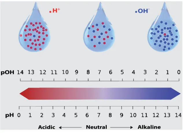
pH value

pH indicates how acidic or basic the water is. Basic water comprises more hydroxyl (OH−) ions while acidic water has extra hydrogen ions (H+). pH ranges from 0 to 14, with 7 being neutral as shown in Figure 3.2. Pure water is neutral, with a pH close to 7.0 at 25^◦C; rainfall has a pH value of around 5.6. pH is normally measured using electrometric and colorimetric methods.

Figure 3.2: Water pH

Low and excessively high pHs can be dangerous for water use. A high pH not only brings a bitter taste in water but also reduces the efficiency of disinfection using chlorine whereas water with a low pH corrodes or dissolves metals and other substances. Also pH is directly proportional to the amount of oxygen in water.

Below are the upshots of pH on other chemicals found in water:

1. Water of lower pH dissolves heavy metals like lead, cadmium, and chromium more easily.

2. The form of some chemicals in water can be changed by changes in the pH thus it may affect animals and aquatic plants. For example, while ammonia is of no harm to fish in acidic or neutral water, it tends to be increasingly more poisonous to fish as the water pH increases.

Water pollution can also change the water pH which in return damages plants and animals that live in that water as shown below:

(34)

1. A slight change in pH affects most aquatic animals and plants that had got used to life in the water of a particular pH.

2. High or very low pH water is lethal; a pH above 10 or below 4 kills most fish, and a limited number of animals can live in water with a pH above 11 or below 3. Also low pH water can irritate fish and aquatic insect gills, reduce the number of hatched eggs for the fish, and damage membranes.

3. Low pH is extremely dangerous to amphibians because of their skin sensitivity to contaminants. Some scientific research has found that the low pH values brought by acid rain has contributed to the current reduction in the population of amphibians globally.

Potability

Potability shows the safety of water for consumption by humans.

3.1 XAI- for- Safe Water Evaluation

3.1.1 Summary

This paper is proposing an Explainable Artificial Intelligence (XAI) approach to water quality prediction. It will help in maintaining water quality or safety within urban centers, improving water management and pollution control and also im- mensely help ecological management organizations of many areas. In this paper, ambiguity of Machine Learning (ML) model predictions is achieved by utilization of feature importance.

3.1.2 Data Preparation and Processing

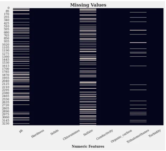
pH and Trihalomethanes are imputed since they have less than 20% missing values.

For the Sulfate feature, as it has more than 20% missing values, some univariate analysis was done on it such that if it is found important, then it too will be imputed or else entirely dropped. The imputation part will happen by setting numeric imputation to true during data setup. Firstly, some univariate analysis on the Sulfate column and the distribution of values for this column is found since values are found to be missing from random indices. From Figure 3.4, the distribution of Sulfate is a little different when the Potability is 0 and when it is 1. So, probably Sulphate has some influence on the Potability, so it will be kept and imputed too.

(35)

Figure 3.3: Missing Values

Figure 3.4: Sulfate Values Distribution

(36)

For feature analysis, data points which were above 95 percentile and below 5 percentile were removed as shown in sample Figure 3.4 . During data set up, outliers were also removed.

Next was looking at how the features influence each other. There does not seem to be any linear relationship between the features as the plots are kind of circular. It can thus be said that there is no multicollinearity but to be 100% sure, the correlation between them was found.

The maximum correlation is 17% (negative) between Sulfate and Solids, it means only 17% variance in the Solids can be explained by Sulfate and vice versa. It seems that there is no multicollinearity, as for it to be present, the correlation should be higher than 80-85% (positive or negative).

3.1.3 Model selection and Description

In this work, 14 classification models were trained say; Extra Trees Classifier, Ran- dom Forest Classifier, Light Gradient Boosting Machine, Quadratic Discriminant Analysis, Gradient Boosting Classifier, Naive Bayes, Logistic Regression, Dummy Classifier, Ada Boost Classifier, Decision Tree Classifier, K Neighbors Classifier, Lin- ear Discriminant Classifier and SVM-Linear Kernel. We then compared them based on various parameters that included Accuracy, AUC ROC score, Recall, Precision, F1 Score, Kappa, MCC and TT (Sec).

Random Forest Classifier

It is a decision trees-based classifier for predicting qualitative responses by dividing the predictor space into different and non-overlapping regions for the same prediction to be made for every observation in that region (majority group) during classification which can be regarded as Bayes classifier. Predictor space is partitioned iteratively based on the highest reduction of some measure of classification error by recursive binary splitting often using the Gini Index,

G=

k

X

k=1

p_mk(1−p_mk₎ (3.1)

where p mk is the quantity of training observations belonging to the k^th class in the m^th region. Over fitting data during learning is addressed by bootstrap driven bagging where the model is trained on the individual bootstrapped training sets to get B classification functions by;

f^∗1(x), . . . , f^∗B(x) (3.2) To average the predictions of all models for the final result as;

f_bag(x) = 1 B

B

X

b=1

f^∗b(x) (3.3)

Observation prediction is done by recording the class prediction by every B tree and summating the predictions with the most frequent class among the B predictions as a majority vote. As extension of bagged trees, random forest aims at model variance reduction by choosing a random sample of the m predictors as split candidates from the full set of p predictors at each split which is given by; m≈√

p thus reducing the total variance of averaged models with a slight increase in bias when decorelating the trees.

(37)

Extra Trees Classifier

This is an ensemble machine learning model that generates several decision trees which are unpruned from the training dataset to enhance prediction. It is convenient at predicting decision trees with regression and classification using majority voting.

Decision Tree Classifier

This Model is generally used for classification problems with both categorical and continuous dependent variables. It has faster training time compared to neural network Models. It is a distribution-free or non-parametric Model, independent of probability dissemination assumptions and can resolve high dimensional data with better accuracy, plus it yields optimal results if deployed with SMOTE.

3.1.4 Model Performance Analysis

To analyze the performance of the trained models, we plotted the AUC ROC Curve, Confusion Matrix, Decision Boundary and Learning Curve.

3.1.5 ML Model Interpretability and Explainability/ Model Interpretation

We interpreted the tree-based models we had trained and selected. For explainability, we utilized an Explainable Artificial Intelligence technique known as SHapley Additive exPlanations (SHAP) . SHAP values show the impact of each feature whose comparative possession yield interpretation of predictions based on baseline values.

SHapley Additive exPlanations (SHAP)

In 2017, Lundberg and Lee published a game theoretical approach that explains ML model outputs by connecting optimal credit portions with related extensions and created an AI framework for SHAP. This average marginal contribution of a feature value out of all possible associations explains the Shapley values, unified measures of feature importance derived from;

φ_i(v) = X

SN{I}

|S|!(|N| − |S| −1)!

|N|! (v(S∪ {i})−v(S) (3.4) where the marginal contribution of the feature [v(S∪i)−v(S)] is computed out of all the subsets S to get the feature Shapley valuei, such that model estimates of all subsets with or without the feature are calculated and added to get the Shapley value as Additive exPlanations of that feature [45]. The plot based on the SHAP values is composed of all training data dots. Descending order is used to reflect the variable feature importance. The level of association effect is illustrated by the horizontal location impact for lower or high predictions. Red color shows high while blue shows low observational correlation of the variables. Local interpretation was also done to explain why the model predicted that particular output as evidenced in the sample SHAP Force Plot. Features that shoot the prediction higher (towards the right side) are displayed in red, while those that push it lower are in blue.

(38)

3.2 XAI- and- EL- for - Water Quality Prediction

3.2.1 Proposed Approach

An overview of the steps we have taken in training our models is summarized in a diagram in Figure 3.5 using an appropriate open global water quality dataset obtained from Kaggle.

Figure 3.5: High Level Diagram for the Proposed Water Quality Prediction Ap- proach

3.2.2 Data Preparation and Preprocessing

At first, we handled the missing values. We found out that the features pH, sulfate and Trihalomethanes had missing values as shown in Figure 3.6. The methods for handling the missing values usually differ depending on the dataset used and the nature of the problem at hand. Our task is to determine water quality based on potability which is a very sensitive matter. Filling in the missing values with certain predicted values can be a very risky decision. For example, if the pH value was originally 0 (zero), that automatically means such water should not be consumed by people. If for some reason, this value has been treated as a missing value and then we go ahead to predict values for it, we would be very wrong. For this reason, we avoided predicting missing values and boldly removed instances with missing values.

(39)

Figure 3.6: Dataset Features with Missing Values

Figure 3.7: Anomaly Plot for the Dataset

Using the pycaret open source library, we then performed anomaly detection to iden- tify the outliers in the dataset as shown in Figure 3.8. The safest way of handling outliers for water safety prediction was removing them since there should not be outliers in the dataset related to life. Over 110 anomalies were observed by evaluating the various dates which reflected the recorded cases that were juggled for water potability. This gave an insight of the potential existence of more instances of juggled cases of undrinkable water as drinkable. On performing datatype verifica- tion of the variables, it was observed that all features were numerical and the target variable was imbalanced.

(40)

Figure 3.8: Outlier Distribution

Next was looking at how the features influence each other, so we visualized the correlation of all features using a heatmap function of Seaborn. There exists no linear relationship between the features that explain the target variable “potability”

as evidenced by the correlation matrix in Figure 3.9. The maximum correlation is 15% (-) for Solids and Sulfates which implies that only 15% variance of Solids can be explained by Sulfates and vice-versa. It can therefore be said that there is no multicollinearity (as for it to be present, the correlation should have been higher than 80-85% (+ or -). The input variables are assumed to be independent implying that we cannot reduce the dimension.

(41)

Figure 3.9: Correlation Matrix

When we applied principle Component Analysis (PCA) to check the explained variance as indicated in Figure 3.10, we observed it would require atleast seven (7) dimensions to explain 90% of the variations. Therefore, dimensionality reduction in this case does not make any change.

Figure 3.10: PCA Plot

(42)

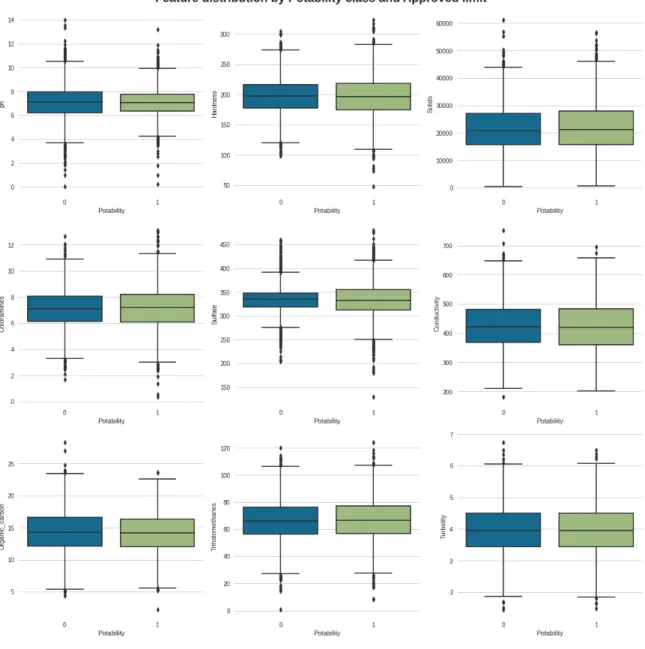
We analyzed the univariate distribution of every predictor variable to better understand the data. Each variable has mostly a normal distribution (the feature means look quite similar with very less difference). Since the graphs are pretty normal, there is no need for normalization. Based on the approved limit in Figure 3.11, we can clearly see the difference in the water classification. For instance; distribution of non-potable water is higher compared to potable water on conductivity, Trihalomethanes and Turbidity. However, pH value, Chloramines, Sulfate, Organic carbon presence does not show significant difference. We hope the hypothetical testing can help us here.

Figure 3.11: Feature distribution by Potability class and approved limit

(43)

Figure 3.12: Features and p-value based on T-test

From the Hypothesis Testing in Figure 3.12 above, we can see that the features Solids and Organic Carbon have significant differences in potable and not-potable water. Other features share similarities between the two classes.

3.2.3 Checking Feature Importance

It is important to note that poor water quality can cause different diseases. There- fore, knowing which features are important when judging water quality will help in making public health decisions. We checked the feature importance of the various water quality metrics based on partial dependencies, mean decrease in impurity and feature permutation. The impurity-based feature importance ranks the most important feature. What basically happens is that at every split (based on the cor- responding feature in each tree), the sum of the decrease in impurity is calculated.

Therefore, the Mean Decrease Gini will be an average of all the tree values. This value increases as the feature becomes important for the model to classify well.

3.2.4 Model Creation

The new clean training dataset was used to train multiple classification algorithms for example Decision Trees, Light gradient Boosting Machine (LGBM), CatBoost, Naive Bayes, Random Forest, Extra Trees, Linear Discriminant Analysis, Gradient Boosting classifier and the Logistic Regression models. Model comparison was performed and explainability done for a few outstanding tree-based classifiers. Then the best models that is; LGBM, CatBoost and Random Forests were ensembled to form a robust water quality prediction model which was trained on the same dataset to assess its binary classification performance before calibration for model generalizability.

(44)

3.2.5 Ensemble Modeling

A soft voting technique was used to ensemble the 3 best models that is; CatBoost, LGBM and Random Forest.

Figure 3.13: Block diagram of Ensemble Learning

Light Gradient Boosting Algorithm (LGBM)

LGBM utilizes decision trees and boosting [16] with a faster training speed and improved efficiency. The algorithm builds on the gradient boosting algorithm by entailing automatic selection of features and boosting larger gradient examples.

LGBM uses histogram-based algorithms which lowers memory usage and applies a more reliable growth strategy known as the best-first which helps greatly in cutting computational costs. It also consists of different model parameters for instance the number of leaves, max depth and boosting type [55] which require tuning. Unfortu- nately, leaf orientation results into overfitting and LGBM prevents this by inclusion of a maximum depth limit to the top of the leaf.

(45)

Categorical Boosting (CatBoost)

CatBoost utilizes the gradient descent framework [1] to predict categorical features.

During model training, several decision trees are consequently constructed to create consecutive trees with relatively lesser loss which in turn constructs a strong learner. The differences between CatBoost and other GBDT algorithms are as follows: Firstly, CatBoost involves combination of categorical features into one by the Feature combinations [37]. Secondly, CatBoost handles categorical features in the training process as opposed to preprocessing and trains the entire dataset. It also uses target statistics to minimize information loss. For regression tasks, CatBoost utilizes the average label value of the dataset in calculating the prior. Thirdly, CatBoost is a fast scorer since it considers decision trees as base predictors [37].

On the other hand, CatBoost algorithm is limited to categorical thus ineffective when it comes to classification data.

H2O AI with StackedEnsemble was also applied which yielded a better accuracy.

Figure 3.14: An example scheme of stacking ensemble learning

(46)

Chapter 4

Results and Recommendations

4.1 XAI- for - Safe Water Evaluation

From Table 4.1 below, Random Forest Classifier achieved the best accuracy, Extra Trees Classifier exhibited a high precision and a great AUC while Decision Trees Classifier achieved the best recall.

Table 4.1: Results Table

Model Accuracy AUC Recall Precision F1 Kappa MCC TT

(Se