DOI: 10.12928/TELKOMNIKA.v14i4.4646 1480
Multi Features Content-Based Image Retrieval Using
Clustering and Decision Tree Algorithm
Kusrini Kusrini*1, M. Dedi Iskandar2, Ferry Wahyu Wibowo3 STMIK AMIKOM Yogyakarta,
Jl. Ringroad Utara Condong Catur Depok Sleman Yogyakarta Indonesia, Telp:+62274884201/fax:+62274884208
*Corresponding author, e-mail: [email protected], [email protected], [email protected]
Abstract
The classification can be performed by using the decision tree approach. Previous researches on the classification using the decision tree have mostly been intended to classify text data. This paper was intended to introduce a classification application to the content-based image retrieval (CBIR) with multi-attributes by using a decision tree. The multi-attributes used were the visual features of the image, i.e. : color moments (order 1, 2 and 3), image entropy, energy and homogeneity. K-means cluster algorithm was used to categorize each attribute. The result of categorized data was then built into a decision tree by using C4.5. To show the concept in application, this research built an application with main features, i.e.: cases data input, cases list, training process and testing process to do classification. The resulting tests of 150 rontgen data showed the training data classification’s truth value of 75.33% and testing data classification of 55.7%.
Keywords: Image, Classification, Decision Tree, Clustering
Copyright © 2016 Universitas Ahmad Dahlan. All rights reserved.
1. Introduction
Image database has been commonly used by many application domains nowadays such as multimedia search engines, digital libraries, medical databases, geographical databases, e-commerce, online tutoring systems and criminal investigations. Image database could be visualized using image browsing as a way to retrieval systems [1]. Image retrieval can be performed using attributes attached to the image such as creation date, storage location, size or other predefined attributes. However, the search performance produced in this way is highly depended on the expertise of a user in describing the image. In addition, the search could not be performed based on the semantics of the image itself [2].
Technology is evolving towards image searching by using method called content-based image retrieval (CBIR) and also known as query by image content (QBIC) [3]. Instead of taking image’s information from external resources or metadata, CBIR approach used the intrinsic features of the image such as color, shape, texture, or a combination of these feature elements [4]. Color as an image feature has been succesfully applied in image retrieval application since it has strong correlation with the objects inside the image [5]. Furthermore, the color feature’s robustness has been proven in processing scaled and orientation-changed images [6-10]. The image itself is classified into three images i.e. intensity image, indexed image, and binary image [11]. To be more specific, CBIR’s retrieval technique is based on information extracted from pixels [12, 13].
CBIR has been widely applied in many research projects. One of application of CBIR is for recognizing porn image [14-15]. CBIR is also used in health area researches. It is used as image administration system that supports the physician task such as diagnosis, telemedicine, teaching and learning new medical knowledge [16-18].
This paper introduces the construction of CBIR by using a case based reasoning concept. In previous research, case-based reasoning has been explained as a concept to build rule for clinical service, specifically in diagnosis problem domain [19]. One algorithm that can be used to build rules as a decision tree is C4.5. It could be also aplied to classify image [20-22].
manually for classification process, the data clustered by using the k-means clustering method. This process is used to classify each of image features before classification process.
2. Research Method 2.1. Architecture System
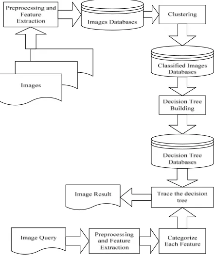
The architecture system of CBIR in this paper was formulated as shown in Figure 1. All of image documents were preprocessed in order to make all images have the same format and size. After the preprocessing step have finished, some visual features were then extracted from the images and stored into image databases. In the next step, using the k-means clustering method [23], each of the features was then categorized and stored into categorized image database. These data were then used to build the decision tree using the C4.5 algorithm.
Figure 1. CBIR Architecture
2.2. Image Feature Extraction
Images were preconditioned into some same states, before the process of feature extraction was started, namely size of 140x140 pixel, bmp format, and turned into 8 bit grey image color mode. The features used in this experiment are quite similar to previous study, that are color moment and texture. The color moment was divided into 3 low-order moments while the texture features used were contrast, correlation, energy, homogeneity, and entropy [24], but in this paper used entropy, energy, contrast, and homogeneity [25]. Entropy, energy, contrast, and homogeneity features represent image texture. Texture can be defined as a region’s characteristic that is wide enough to form pattern repetition. In another definition, texture is defined as a specifically ordered pattern consisting of pixel structures in the image.
One parameter needed to calculate the value of entropy, energy, contrast, and homogeneity is obtained from co-occurence matrix, that is a matrix that describes the frequency with which a pair of two pixels with a certain intensity within a certain distance and direction occurs in the image. Co-occurrence intensity matrix p (i1, i2) is defined by the following two simple steps:
2. Count the number of pixel pairs that have intensity values of i1 and i2 and distance of d pixels.
Put the calculation of each pair intensity values into the matrix according to the coordinates, which the abscissa for intensity value i1 and the ordinate for intensity value i2.
Entropy is an image feature used for measuring the disorder of intensity distribution. The entropy calculation is shown in Equation 1.
1 2 (1, 2)log (1, 2)
i i pi i pi i
Entropy (1)
Energy is a feature for measuring the number of concentration of intensity pairs in co-occurrence matrix. Equation 2 is used to calculate this feature’s value. The value will be increased if qualified pixel pairs that matched the co-occurrence intensity matrix requirement are more concentrated at some coordinates of the matrix and will be decreased if they are more dispersed.
Energy i p2(i1,i2 )
2
i1
(2)
The contrast feature is used to measure the strength of different intensity of the image, while homogeneity is used to measure homogeneity of image intensity variation. Image’s homogeneity value will be increased as its variation intensity is decreased. The formula to measure the image contrast is shown in Equation 3 while that for measuring the homogeneity is shown in Equation 4.
Contrast i (i1i2 )2p(i1,i2 )
2
i1
(3)
Homogeneity p(i1,i2 )
1|i1i2 | i2
i1
(4)
The notation of p in Equation 2, 3 and 4 denotes the probability and has value in the range of 0 to 1, that is the element value in co-occurrence matrix. Meanwhile i1 and i2 are
denoted as nearby intensity pair in the x and y direction.
Given a sample of 1-bit image data with a size of 3 x 3 pixels. Finding the mean of RGB values of each pixel, the result is represented in a matrix as shown in Figure 2.
Figure 2. Image’s RGB mean matrix
Feature calculations of entropy, energy, contrast and homogeneity is based on the occurrence intensity matrix. Consequently, prior to searching those features values, co-occurrence intensity matrix is needed to be built. In this system, the value of distance (d)=1 and direction in angle 45o (dx=1 and dy=1) are predetermined. From the above setting, then the value of co-occurrence intensity matrix value from image matrix Figure 2 is obtained as shown in Figure 3.
Figure 3. Co-occurrence Intensity Matrix Figure 4. Illustration of pair count calculation
The value of p(0,1) is obtained from element value on row dx=0 and column dy=1 divided by total element value in co-occurrence matrix. Thus, the value of p(0,1) is ¼ or 0.25.
The entropy visual feature value is calculated by Equation 1, as follows:
entropy =-((p(0,0)log(p(0,0)+(p(0,1)log(p(0,1)+(p(1,0)log(p(1,0)+ (p(1,1)log(p(1,1)
=-(0.25 log(0,25)+0.25 log(0.25)+0 log(0)+0.5 log(0.5) =-(- 0.15 - 0.15 – 0 - 0.15)
=0.45
The value of energy visual feature is calculated by Equation 2, as follows:
energy
=(p2(0,0) p2(0,1) p2(1,0) p2(1,1))= (0.2520.252020.52) = 0.375
The value of visual feature contrast is obtained with calculation using Equation 3. That is:
contrast
=(00)20.25(01)20.25(10)20(11)20.5 = 0 + 0.25 + 0 + 0= 0.25
Visual feature homogeneity is obtained with calculation using Equation 4. That is:
Homogeneity =
1 5 . 0 2 0 2 25 . 0 1 25 . 0
= 0.25 + 0.125 + 0.125 + 0.5
= 0.875
Color moment can be defined as simple representation of color feature in colored images. The three low-order moments of color for capturing the information of image’s color distribution are mean, standard deviation and skewness [25]. For a color c in the image, the mean of c is symbolized as μc, the standard deviation as σc and the skewness as θc. The
values of μc, σc, and θc are calculated using Equation 5, Equation 6, and Equation 7,
respectively. M i N j c ij p MN c 1 1 1
(5)
2 1 1 1 2 ) ( 1
M i N j c c ij p MN c (6)
3 1 1 1 3 ) ( 1
M i N j c c ij p MN c Where M and N are the horizontal and vertical sizes of the image and is the value of color c in the image’s row i and column j.
Using Equation 5, the value of visual features color moment order 1 is calculated from the matrix as follows:
c
=(
0
1
1
1
0
1
1
1
1
)
3
3
1
x
= 0.78
The value of color moment order 2 is obtained using the following steps:
1. Transform each value in the RGB mean matrix in Figure 2 by operating each value in the matrix with the Equation 8.
2
)
(
p
ijc cnb
(8)c ij
p
is the matrix cell’s value in row i and column j and nb is the new value of the cell. The result is then represented in Figure 5.Figure 5. Color Moment Order 2 Value Matrix
Figure 6. Color Moment Order 3 Matrix
2. The color moment order 2 value
c is calculated from the matrix using Equation 2.c
= 21 1 1 1
M i N j nb MN c
= 21 556 . 1 3 3 1
x = 0.416The color moment order 3 value is obtained with the following steps:
1. Transform each value in the RGB mean matrix in Figure 2 by operating each value in the matrix with the Equation 9.
3
)
(
p
ijc cnb
(9)c ij
p
is the matrix cell’s value in row i and column j and nb is the matrix new cell’s value. Using these calculations, the matrix in Figure 2 will be transformed into the color moment order 3 matrix as shown in Figure 6.2. The color moment order 3 value
c is calculated from the matrix using Equation 3.c
= 31 864 . 0 3 3 1
x = -0.4582.3. K-Mean Clustering
Clustering machine is intended to map the continous or discrete class data with many variations into discrete class with determined variations. The input of this process is:
1. Initial data, that can be either continuous or discrete data.
2. Delta, that is the value to be used to determine the allowed gap between centroid and mean. The output of this process is a mapping table containing the discrete class including its centroid value.
The algorithm used in the data clustering machine is derived and extended from k-means clustering algorithm. This data clustering using the K-Means method is commonly done with basic algorithm as follow [26]:
1. Determine count of class (cluster) 2. Determine initial centroid of each class
3. Put each data into class which has the nearest centroid 4. Calculate the data mean from each class
5. For all class, if the difference of the mean value and centroid goes beyond tolerable error, replace the centroid value with the class mean then go to step 3.
In fundamental k-means clustering algorithm, initial centroid value from specific discrete class is defined randomly, while in this research the value is produced from an equation shown in Equation 10.
n n i i c * 2 min) (max min) (max * ) 1 (
min
(10)
Where,
ci :centroid class i
min : the lowest value of continue class data max : the biggest value of discrete class data n : total number of discrete class
The building process of discrete class is shown as follows: 1) Specify the source data; 2) Specify desired total number of discrete class (n); 3) Get the lowest value from source data (min); 4) Get the highest value from source data (max); 5) Specify delta (d) to get the acceptable error by Equation 11; 6) For each discrete class, find the initial centroid (c) by Equation 10; 7) For each value in source data, put it into its appropriate discrete class, which is one that has nearest centroid to the value; 8) Calculate the average value of all members for each class (mean); 9) For each discrete class, calculate the difference between its mean and its centroid (s) by Equation 12; 10) For each discrete class, if s>e , then replace its centroid value with its mean, put out all values from their corresponding class then go back to step 7.
ed* (maxmin) (11)
n i i i c mean s 1 || (12)
2.4. C4.5 Algorithm
Decision tree is one of methods in classification process. In decision tree, classification process involving classification rules generated from a set of training data. The decision tree will split the training data based on some criteria given. The criteria are divided into target criteria and determinator criteria. The classification process produces the target criteria values based on determinator criteria values [27].
the algorithm is creating branches based on the values inside of the criterion. The training data then categorized based on values at the branch. If the data considered homogen after the previous step, then the process for this branch is immediately stopped. Otherwise, the process will be repeated by choosing another criterion as next root node until all the data in the branch are homogen or there is no remain deciding criterion can be used.
The resulting tree will then be used in classification of new data. The proccess of classification is conducted by matching the criterion value of the new data with the node and branch in decision tree until finding the leaf node which is also the target criterion. The value at that leaf node is being the conclusion of classificion result.
Using C4.5 algorithm, choosing which attribute to be used as a root is based on highest gain of each attribute, the gain is counted using Equation 13 and 14 [28].
n
i
Si Entropy S
i S S Entropy A
S Gain
1
) ( *
| |
| | ) ( )
,
( (13)
n
i pi pi
S Entropy
1 *log2 )
( (14)
Where
S : Case set
A : Attribute
n : Partition Count of attribute A |Si| : Count of cases in ith partition |S| : Count of cases in S
pi : Proportion of cases in S that belong to the i th
partition
3. Results and Analysis 3.1. Result
The result of this research is a computer program to classify images. The program’s main features are 1) Data Case Input; 2) Case List; 3) Training Process; and 4) Testing Process.
3.1. Data Input and Case List
The Data Case Input feature is used to store images that will be used in the training process. In this feature, the program will do preprocessing, take the image visual feature’s values and then store them in the database. The case data input feature interface is shown in Figure 7. This figure shows that the loaded image processed to some visual features as explained in section 2.2 and the classification text box is filled manually as the expert judgement.
The Case List feature is used to review the cases stored in the database. This feature is also provided with ability to delete a particular data that are assumed not to be used in the next training process. The Case List page is shown in Figure 8.
Figure 8. List of Cases Feature
3.2. Training Process using K-Means Cluster and C4.5 Algorithm
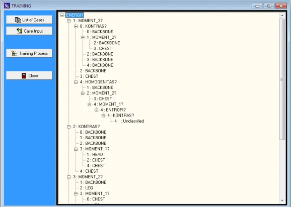
The training process is used to produce the decision tree from the cases in the case list. This process contains 2 sub processes, they are categorization process and decision tree building process. The categorization process is performed for each of image visual feature by using K-Means Cluster algorithm as explained in section 2.3. The input of categorization process is all values of images in a features and the result is the cluster and the centroid of each data. The cluster selected will be the one that has the nearest centroid. The decision tree building process is performed using C4.5 algorithm. The training process is then visualized in the form of decision tree as in Figure 9 and in a table of rule as shown in Figure 10.
Figure 10. List of Rules Feature
3.3. Testing Process
The testing feature is used to do classification to newly incoming images. The classification is carried out by comparing between the new image’s visual feature value and the rule constructed in the prior training process. The testing feature is shown in Figure 11.
Figure 11. Testing Feature
3.2. Analysis
The testing process was carried out with 150 rontgen image data and resulted some classifications. The data is shown in Table 1.
Table 1. Cases Classification
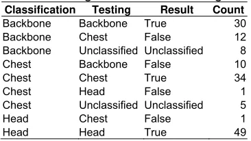
The testing was carried out by comparing between the classification from system’s output and the expert judgment in Case Input Data as explained in section 3.1. The testing to all training data resulted to true classification for 113 data. It means 75.3% of truth value. The detail result of testing training data is shown in Table 2.
Table 2. Testing Result of All Training Data
Classification Testing Result Count
Backbone Backbone True 30
Backbone Chest False 12
Backbone Unclassified Unclassified 8
Chest Backbone False 10
Chest Chest True 34
Chest Head False 1
Chest Unclassified Unclassified 5
Head Chest False 1
Head Head True 49
Beside the testing process to all training data, it is also conducted 10 experiments using 120 data. The data consists of 40 Backbone, 40 chest, and 40 head image data with different combination. The test result is shown in Table 3.
Table 3. Testing Results of the 120 Training Data
Iteration True False Unclassified
1 88 22 10
2 88 23 9
3 85 25 10
4 85 25 10
5 88 23 9
6 92 19 9
7 97 15 8
8 97 17 6
9 94 19 7
10 90 20 10
Average 90.4 20.8 8.8
% 75.33 17.33 7.33
The testing to testing data was done by 10-fold cross validation. It is used 120 training data and 30 testing data for each of experiments. The test result with this model is shown in Table 4. From the Table 4, it is known that the testing process to the data test producing correct classification of 55.7% wrong classification of 33.7% and unclassified data about 10.7%.
Table 4. Testing Results of the Test Data
Iteration True False Unclassified
1 14 16 0
2 20 6 4
3 20 9 1
4 18 9 3
5 16 7 7
6 16 9 5
7 16 11 3
8 16 9 5
9 19 7 4
10 12 18 0
Average 16.7 10.1 3.2
In order to compare the result, the same dataset is tested into classification algorithm without clustering preprocessing. This time, the class range is defined manually. The testing to all training data resulted to true classification for 23 data. It means 15.3% of truth value. The result of 10 experiments using 120 training data with different combination without clustering process is shown in Table 5.
Table 5. Testing Results of the 120 Training Data Without Clustering Process
Iteration True False Unclassified
1 17 20 83
2 20 18 82
3 21 17 82
4 20 17 83
5 18 17 85
6 19 19 82
7 20 19 81
8 17 16 87
9 16 15 89
10 16 18 86
Average 18,4 17,6 84
% 15,3 14,7 70
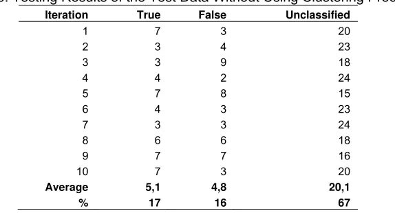
The result of testing to testing data that was done by 10-fold cross validation that is not using clustering process. The result is shown in Table 6. From the Table 6, it is known that the testing process to the data test without clustering process producing correct classification of 17% wrong classification of 16% and unclassified data about 67%.
Table 6. Testing Results of the Test Data Without Using Clustering Process
Iteration True False Unclassified
1 7 3 20
2 3 4 23
3 3 9 18
4 4 2 24
5 7 8 15
6 4 3 23
7 3 3 24
8 6 6 18
9 7 7 16
10 7 3 20
Average 5,1 4,8 20,1
% 17 16 67
Comparing the above processes of classification with and without clustering algorithm, it shows that the using of clustering can increase the accuracy of classification process. Since it is done manually, the classification without clustering algorithm is less accurate to define the class range based on data distribution.
4. Conclusion
Based on the conclusion, there are some opportunities and challenges for further researches to improve this research, among others determining the classification of data which are still in unclassified category in order to get a better accuracy value and examining other visual features that are able to increase classification accuracy value.
References
[1] Schaefer G. Interactive Browsing of Large Image Databases. IEEE Conference - Sixth International Conference on Digital Information Processing and Communications (ICDIPC). Beirut. 2016: 168-170. [2] Karmakar S, Dey S, Sahoo S. Towards Semantic Image Search. IEEE Tenth International
Conference on Semantic Computing (ICSC). California. 2016: 483-487.
[3] Ambika P, Samath JA. Visual Query Exploration Process and Generation of Voluminous Image Database for CBIR Systems. IEEE Conference – Third International Conference on Computing Communication & Networking Technologies (ICCCNT). Coimbatore. 2012: 1-7.
[4] Jyothi B, Latha YM, Reddy VSK. Relvance Feed Back Content Based Image Retrieval Using Multiple Features. IEEE International Conference on Computational Intelligence and Computing Research (ICCIC). Coimbatore. 2010: 1-5.
[5] Minarno AE, Kurniawardhani A, Bimantoro F. Image Retrieval Based on Multi Structure Co-Occurence Descriptor. TELKOMNIKA Telecommunication Computing Electronics and Control. 2016; 14(3): 1175-1182.
[6] Guizhi Li. Improving Relevance Feedback in Image Retrieval by Incorporating Unlabelled Images. TELKOMNIKA Indonesian Journal of Electrical Engineering. 2013; 11(7): 3634-3640
[7] Sreedhar J, Raju SV, Babu AV. Query Processing for Content Based Image Retrieval. International Journal of Soft Computing and Engineering. 2011; 1(5): 122-131.
[8] Patil C, Dalal V. Content Based Image Retrieval Using Combined Features. International Conference & Workshop on Emerging Trends in Technology. New York. 2011; 11: 102-105.
[9] Alnihoud J. Content-Based Image Retrieval System Based on Self Organizing Map, Fuzzy Color Histogram and Substractive Fuzzy Clustering. The International Arab Journal of Information Technology. 2012; 9(5): 452-458.
[10] Haridas K, Thanamani AS. Well-Organized Content Based Image Retrieval System in RGB Color Histogram, Tamura Texture and Gabor Feature. International Journal of Advanced Research in Computer and Communication Engineering. 2014; 3(10): 8242-8248.
[11] Sai NST, Patil RC. Image Retrieval Using Bit-Plane Pixel Distribution. International Journal of Computer Science & Information Technology(IJCSIT). 2011; 3(3): 159-174.
[12] Hussain SJ, Kumar RK. A Novel Approach of Content Based Image Retrieval and Classification using Fuzzy Maps. International Journal of Research Studies in Computer Science and Engineering. 2015; 2(3): 91-94.
[13] Youness C, Khalid EA, Mohammed O. New Method of Content Based Image Retrieval based on 2-D ESPRIT Method and the Gabor Filters. Indonesian Journal of Electrical Engineering and Computer Science. 2015; 15(2): 313-320.
[14] Liu Y, Xiao C, Wang Z, Bian C. An One-Class Classification Approach to Detecting Porn Image. Conference on Image and Vision Computing. New York. 2012; 27: 284-289.
[15] Karavarsamis S, Pitas I, Ntarmos N. Recognizing Pornographic Images. Multimedia and Security. New York. 2012; 12: 105-108.
[16] Ramu B, Thirupathi D. A new methodology for diagnosis of appendicitis using sonographic images in image mining. International Conference on Computational Science, Engineering and Information Technology. New York. 2012; 2: 717-721.
[17] Kumar A, Nette F, Klein K, Fulham M, Kim J. A Visual Analytics Approach Using the Exploration of Multidimensional Feature Spaces for Content-Based Medical Image Retrieval. IEEE Journal of Biomedical and Health Informatics. 2015; 19(5): 1734-1746.
[18] Ramos J, Kockelkorn TTJP, Ramos I, Ramos R, Grutters J, Viergever MA, Ginneken BV, Campilho A. Content-Based Image Retrieval by Metric Learning From Radiology Report: Application to Interstitial Lung Diseases. IEEE Journal of Biomedical and Health Informatics. 2016; 20(1): 281-292. [19] Haolin Gao. Which Representation to Choose for Image Cluster. TELKOMNIKA Indonesian Journal
of Electrical Engineering. 2014; 12(8): 6181-6189
[20] Kusrini. Klasifikasi Citra dengan Pohon Keputusan. Jurnal Ilmiah Teknologi Informasi (JUTI). 2008; 7 (2): 47-56.
[21] Kusrini, Harjoko, A. Decision Tree as Knowledge Management Tool for Image Classification. Knowledge Management International Conference. Malaysia. 2008: 190-195.
[22] Kusrini. Differential Diagnosis Knowledge Building by using CUC-C4.5 Framework. Journal of Computer Science(JCS). 2010; 6(2): 180-185.
[24] Chaugule A, Mali SN. Evaluation of Texture and Shape Features for Classification of Four Paddy Varieties. Journal of Engineering. 2014; 2: 1-8.
[25] Dubey RS, Choubey R, Bhattacharjee J. Multi Feature Content Based Image Retrieval. International Journal on Computer Science and Engineering(IJCSE). 2010; 2(6): 2145-2149.
[26] Masruro A, Wibowo FW. Intelligent Decision Support System For Tourism Planning Using Integration Model of K-Means Clustering and TOPSIS. International Journal of Advanced Computational Engineering and Networking. 2016; 4(1): 52-57.
[27] Agrawal GL, Gupta H. Optimization of C4.5 Decision Tree Algorithm for Data Mining Application. International Journal of Emerging Technology and Advanced Engineering. 2013; 3(3): 341-345. [28] Dai W, Ji W. A MapReduce Implementation of C4.5 Decision Tree Algorithm. International Journal of