CHAPTER 12
THE
F
DISTRIBUTION
Definition
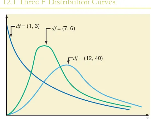
1. The F distribution is continuous and skewed to the right. 2. The F distribution has two numbers of degrees of
freedom: df for the numerator and df for the denominator.
Example 12-1
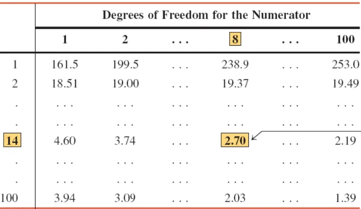
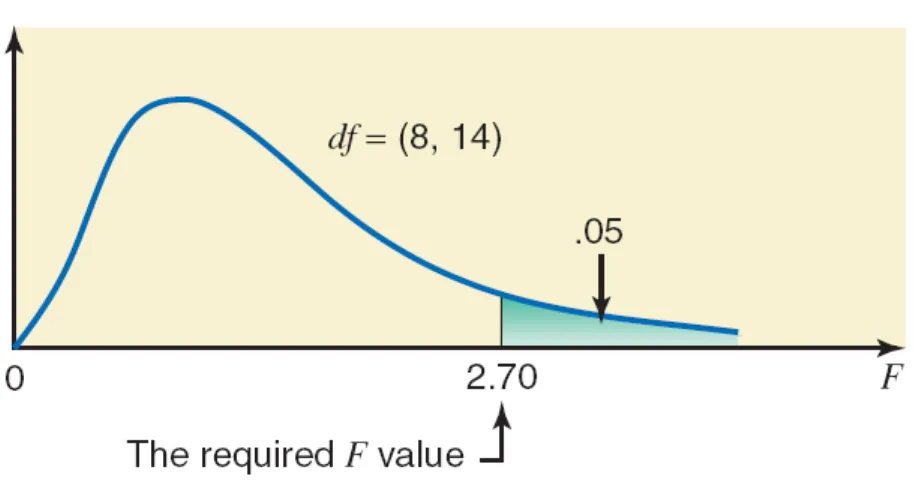
Find the F value for 8 degrees of freedom for the numerator,
Figure 12.2 The critical value of
F
for 8
df
for the numerator, 14
df
ONE-WAY ANALYSIS OF VARIANCE
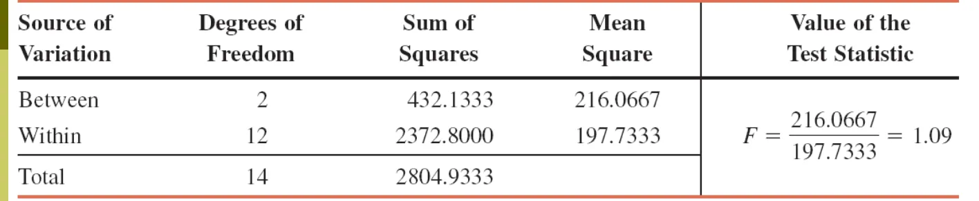
Calculating the Value of the Test Statistic
ONE-WAY ANALYSIS OF VARIANCE
Definition
ANOVA is a procedure used to test the null hypothesis that
Assumptions of One-Way ANOVA
The following assumptions must hold true to use one-way
ANOVA.
1. The populations from which the samples are drawn are (approximately) normally distributed.
2. The populations from which the samples are drawn have the same variance (or standard deviation).
Calculating the Value of the Test Statistic
Test Statistic F for a One-Way ANOVA Test
The value of the test statistic F for an ANOVA test is
calculated as
The calculation of MSB and MSW is explained in Example
12-2.
Variance between samples
MSB
or
Variance within samples
MSW
Example 12-2
Example 12-2
Calculate the value of the test statistic F. Assume that all the
Example 12-2: Solution
Let
x = the score of a student
k = the number of different samples (or treatments)
ni = the size of sample i
Ti = the sum of the values in sample i
n = the number of values in all samples
= n1 + n2 + n3 + . . .
Σx = the sum of the values in all samples
= T1 + T2 + T3 + . . .
Example 12-2: Solution
To calculate MSB and MSW, we first compute the
between-samples sum of squares, denoted by SSB and the within-samples sum of squares, denoted by SSW. The sum of
SSB and SSW is called the total sum of squares and is denoted by SST; that is,
SST = SSB + SSW
Between- and Within-Samples Sums of Squares
The between-samples sum of squares, denoted by SSB,
is calculated as
2 2
2 2
3
1 2
1 2 3
(
)
...
x
T
T
T
SSB
n
n
n
n
=
+
+
+
−
Between- and Within-Samples Sums of Squares
The within-samples sum of squares, denoted by SSW, is
calculated as
2
2 2
2 1 2 3
1 2 3
...
T
T
T
SSW
x
n
n
n
=
−
+
+
+
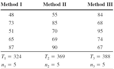
Example 12-2: Solution
∑x = T
1 + T2 + T3 = 324+369+388 = 1081
n = n
1 + n2 + n3 = 5+5+5 = 15
Σx² = (48)² + (73)² + (51)² + (65)² + (87)² + (55)² +
Example 12-2: Solution
2 2 2 2
2 2 2
(324)
(369)
(388)
(1081)
SSB
432.1333
5
5
5
15
(324)
(369)
(388)
SSW
80,709
2372.8000
5
5
5
SST
432.1333 2372.8000
2804.9333
Calculating the Values of MSB and MSW
MSB and MSW are calculated as
where k – 1 and n – k are, respectively, the df for the
numerator and the df for the denominator for the F
distribution. Remember, k is the number of different
samples.
and
1
SSB
SSW
MSB
MSW
k
n
k
=
=
Example 12-2: Solution
432.1333
216.0667
1
3
1
Example 12-3
Reconsider Example 12-2 about the scores of 15
fourth-grade students who were randomly assigned to three groups in order to experiment with three different methods of
teaching arithmetic. At the 1% significance level, can we reject the null hypothesis that the mean arithmetic score of all fourth-grade students taught by each of these three
methods is the same? Assume that all the assumptions
Example 12-3: Solution
Step 1:
H
0: µ1 = µ2 = µ3
(The mean scores of the three groups are all equal)
H
1: Not all three means are equal
Step 2:
Because we are comparing the means for three normally
distributed populations, we use the F distribution to make this
Example 12-3: Solution
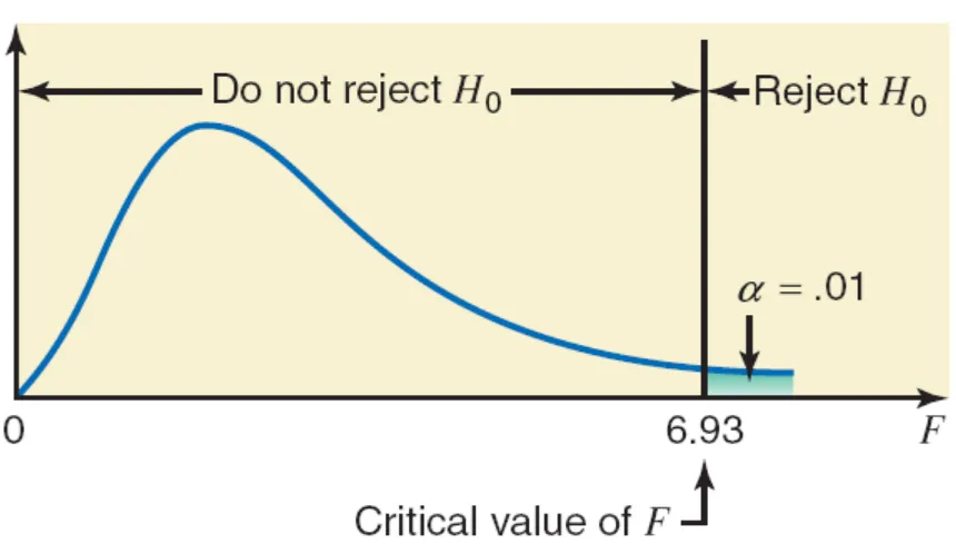
Step 3:
α = .01
A one-way ANOVA test is always right-tailed Area in the right tail is .01
df for the numerator = k – 1 = 3 – 1 = 2
Example 12-3: Solution
Step 4 & 5:
The value of the test statistic F = 1.09
It is less than the critical value of F = 6.93
It falls in the nonrejection region
Hence, we fail to reject the null hypothesis.
Example 12-4
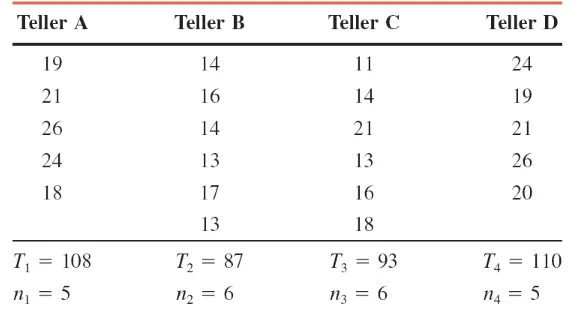
From time to time, unknown to its employees, the research department at Post Bank observes various employees for their work productivity. Recently this department wanted to check whether the four tellers at a branch of this bank serve, on average, the same number of customers per hour. The research manager observed each of the four tellers for a
certain number of hours. The following table gives the number of customers served by the four tellers during each of the
Example 12-4
At the 5% significance level, test the null hypothesis that the
mean number of customers served per hour by each of these four tellers is the same. Assume that all the assumptions
Example 12-4: Solution
Step 1:
H0: µ
1 = µ2 = µ3 = µ4
(The mean number of customers served per hour by each of the four tellers is the same)
Example 12-4: Solution
Step 2:
Because we are testing for the equality of four means for four normally distributed populations, we use the F
Example 12-4: Solution
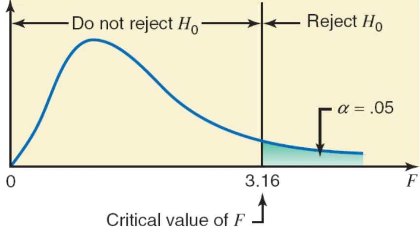
Step 3:
α = .05.
A one-way ANOVA test is always right-tailed. Area in the right tail is .05.
df for the numerator = k – 1 = 4 – 1 = 3
Example 12-4: Solution
Step 4:
Σx = T
1 + T2 + T3 + T4 =108 + 87 + 93 + 110 = 398
n = n
1 + n2 + n3 + n4 = 5 + 6 + 6 + 5 = 22
Σx² = (19)² + (21)² + (26)² + (24)² + (18)² + (14)² +
Example 12-4: Solution
(
)
22
2 2 2
3
1 2 4
1 2 3 4
2 2 2 2 2
2
2 2 2
2 1 2 3 4
1 2 3 4
2 2 2 2
(108) (87) (93) (110) (398)
255.6182
5 6 6 5 22
(108) (87) (93) (110)
7614 158.2000
5 6 6 5
x T
T T T
SSB
n n n n n
T
T T T
SSW x
n n n n
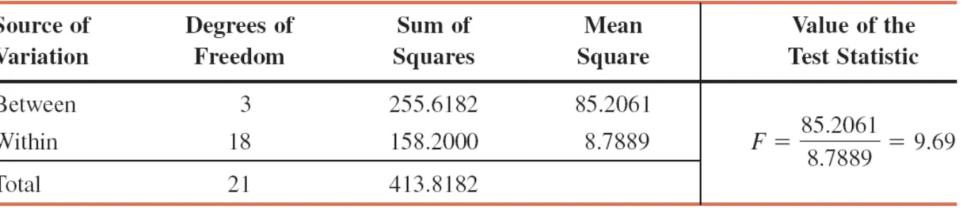
Example 12-4: Solution
255.6182
85.2061
1
4
1
Example 12-4: Solution
Step 5:
The value for the test statistic F = 9.69
It is greater than the critical value of F = 3.16
It falls in the rejection region
Consequently, we reject the null hypothesis