BAYESIAN SURVIVAL MIXTURE MODEL
ON YEARS OF SCHOOLING IN
WEST PAPUA PROVINCE
Maulidiah Nitivijaya, Nur Iriawan, Heri Kuswanto
Department of Statistics, Institut Teknologi Sepuluh Nopember,
Surabaya, Indonesia
[email protected] (Maulidiah Nitivijaya)
Abstract
Education could be considered as one of the basic pillars to determine the performance
indicator of a respective region. Year of schooling is one of the education indexes,
which becomes the government's target in the 9-year compulsory education program.
This index illustrates the importance of knowledge and higher-level skills. Meanwhile,
West Papua Province as one of the youngest provinces in Indonesia is challenged to
improve the quality of human resources, particularly in the underdeveloped regions.
Therefore, it is important to identify the variables which influence the years of
schooling in the West Papua province. Statistically, the type of data such as length of
time is frequently used to be the survival analysis. Nevertheless, the distribution pattern
of the response variables is difficult to be analyzed. For that reason, this study applied
mixture model on years of schooling. Mixture model estimation leads to the complex
statistical problems with a number of parameters. Bayesian methods accomplish the
estimation through the simulation process of Markov Chain Monte Carlo (MCMC). The
survival mixture model was formed based on the status of county. Rural areas were
evidenced to give the contribution of years of schooling distribution more than urban area up
to 59.87 percent. The opportunity to obtain formal education at least to junior high school in
urban areas was greater than rural area had, yet it went down faster in year 12-th or in senior
high school level. In general, the factors which influenced the years of schooling in urban and
rural areas turned out to be different.
Keywords: mixture survival, MCMC, Cox regression, years of schooling.
Presenting Author's biography
1.
Introduction
One of the ways to build a modern developed nation is by improving the quality of education. Education is a lifelong learning process to establish good character, to develop the potential and individual talents, as well as to invest a brighter life. Education is one of the indicators in the calculation of the Human Development Index (HDI). National Socioeconomic Survey (Susenas) 2014 showed that the HDI of Indonesia is still moderate. In fact, there were provinces with low HDI, one of them was West Papua Province. West Papua had an education index ranked on five lowest at the national level. Mean years of schooling (MYS) of West Papua amounted to 8.66 in 2014 which means that the most population has not been reached to junior high school.
This level is very low compared to a target of the 9-year compulsory education program. In order to improve the quality of education, it is necessary to study about the factor affecting MYS. The research about educational attainment showed that it was affected by student-teacher ratio and education of parents [1]. Furthermore, MYS was also influenced by the age, employment, education of householder, expenditure per capita, topography, the numbers of household members, householder’s occupation, status of county, and marital status [2, 3].
In general, survival analysis is a statistical procedure to study the case which the outcome variable of interest is time or failure event. Survival time is started from the beginning treatment until occurs the interest of response. Cox proportional hazards regression is one of the survival analysis methods that involve predictor variables. Frequently, there is a data distribution pattern, by which the response variable is difficult to be observed visually by histogram. The pattern generates a typical model which appears from an observed data set and should identify the sub-population or group, known as a mixture model [4]. Many mixture models have been developed in survival analysis by a Bayesian approach. Bayesian survival mixture model has been widely applied in social, education, and other field. In this study, Bayesian survival mixture model was applied to examine years of schooling in West Papua based on status of county and the affected factors especially for the young people (16-24 years old).
2.
Methods
2.1.Survival AnalysisEssentially, the first step in the survival analysis is the estimation of the distribution of failure times. The response variable in survival analysis is an observation time until occur a failure event. Distribution testing of the response variable (goodness of fit) can be done by several ways, such as by using the Anderson Darling test. The Anderson Darling test statistic is defined as follows:
( )
(
)
2
1 1
1
(2
1) ln
ln(1
)
,
n
n i i n i
i
A
F x
F x
n
n
= + −
= −
−
+
−
−
∑
(1)where F is the cumulative distribution function of the specified distribution and the xi are the ordered
data, with the hypothesis as below:
H0 : the data follow a specified distribution
H1 : the data do not follow the specified distribution.
H0 is rejected if An2 is larger than a critical value. The data follow a particular distribution if the
Anderson-Darling statistic getting smaller [5].
There are three points that must be considered in determining the survival time, namely: time origin or the time the study started early, failure time and measurement scale of time [8]. Therefore, the survival analysis allows for objects that are not observed in full until failure occurs or the event called censored data. Generally, there are three reasons for censoring, such as: lost to follow up, if the object of observation died, moved away, or refuse to be inspected; drop out if the treatment should be discontinued for any reason; and termination of study that if the study period ends while the object of observation has not been reached in the event of failure.
In the analysis of survival, survival time is performed in three functions, namely: probability density function, survival function and hazard function. Survival function S(t) can be defined as the probability that an experimental subject from the population will have a lifetime exceeding t and is expressed by the following equation,
( ) Pr( ) 1 Pr( ) 1 ( )
S t = T ≥ = −t T < = −t F t . (2)
Hazard function h (t) is a shortly reaction or failure rate moment when a person come through an event in time t. A relationship between the survival, hazard and probability density function for survival time is as follows
( )
( )
,
( )
f t
h t
S t
=
(3)whereas the relationship between the cumulative hazard function denoted H(t) with a survival function denoted S(t) is
( ) ln ( )
H t = − S t . (4)
The Cox proportional hazard model is usually written in terms of the hazard model as below,
( )
0( )
exp(
1 1)
.i i p pi
h t =h t
β
x +…+β
x (5)Odds ratio in hazard function is the measure used to determine the tendency or risk, in other words; it shows a ratio between individual odd in success category of predictor variable (x = 1) and failure category (x = 0) [9] or can be written,
(
)
(
)
( )
( )
( )
( )
.1
0 0
.0
0 0
|
1
,
|
0
h t x
h t e
h t e
e
h t x
h t e
h t
β β
β β
=
=
=
=
=
(6)which means that the failure rate of individual with category x = 1 is equal to �� times the failure rate of individual with category x = 0.
2.2.Mixture Model and Bayesian Approach
Mixture model is a typical model of which can be seen from the observed data that is structured by some subpopulations or groups. Mixture distributions comprise a finite or infinite number of components, possibly of various distribution types, that can describe different features of data [10]. Suppose there are K components in a mixture, given f1(x), f2(x), ..., fK(x) as the first component of
density, the second until K components respectively, then the model mixture composed by K components will be written as follows:
1 1 2 2
( | )
( )
( ) ...
K K( ),
f x
π
=
π
f x
+
π
f x
+ +
π
f
x
(7)where
�
1 is the contribution of the first mixture component,�
2 is the second component, and�
�is
the contribution of the K-th mixture component, and �1+�2+⋯+��= 1.
[12]. The likelihood function of mixture distribution is unusual with the univariate distribution. The likelihood function of a mixture model based on Eq. (7) is
(
)
1
|
n
mix mix i
i
f
l x
θ
=
=
∏
(
)
(
)
(
)
1 2
1 2
1 1 1 2 2 2
1 1 1
| | | ,
K
k
n n n
mix i i K iK K
i i i
f x f x f x
l
λ
θ
λ
θ
λ
θ
= = =
=
∏
+∏
+…+∏
(8)where n1+n2+ ...+ nK = n and K is the number of mixture component. The estimation of a mixture
model which has many parameters would bring complexities. To resolve the computational difficulties, the Bayesian approach has an advantage of drawing conclusions numerically, by using Markov chain Monte Carlo (MCMC) [13]. In the Bayesian approach, the sample data obtained from the population also taking into account an initial distribution of the so-called prior. In contrast to the classical statistic approach (frequentist) which supposes the parameter as fixed, a Bayesian approach considers the parameters as random variables that have a distribution as the prior distribution. From the prior distribution can be determined the posterior distribution to obtain the Bayesian estimators. Bayesian theorem is based on the posterior distribution which is a combination of prior distributions (past information prior to observation) and observation data used to compile a likelihood function [14]. If there is a given parameter θ by the observation x, then the posterior probability distribution of
θ given x will be proportional to the multiplication of the prior distribution θ and a likelihood function of x given θ. The formula can be expressed as follows
( )
|( )
| ( ).f θx ∝ f xθ f θ (9)
The specification of the prior distribution is very important in Bayesian methods because the prior distribution affects the posterior forms that will be used to make decisions. There are several types of prior distributions in Bayesian methods, include: prior or non-conjugate priors, namely the determination of prior based on the pattern likelihood of data; proper or improper priors (Jeffrey’s prior) that is associated with the allocation of prior weight or density at any point whether or not uniformly distributed; informative or non-informative priors that determination based on the availability of knowledge or information about the distribution pattern from the previous studies; pseudo prior describes the determination prior which is comparable to the results of an elaboration frequentist way [14,15,16].
In Bayesian analysis, by using MCMC method can simplify the analysis so that the decisions from the results will be done quickly and accurately. MCMC approaches reduce the computational load effectively in completing the complex integration of equations and bring through a simulation process by taking a random sample of the complicated stochastic model [16]. The basic idea of the MCMC is generating the sample data from the posterior distribution correspond Markov chain process by using Monte Carlo simulation iterative in order to obtain the convergent conditions in the posterior.
One of MCMC techniques for estimating the model parameter is the Gibbs sampling. Gibbs sampling can be defined as a simulation technique to generate random variables of a particular distribution function without having to calculate the density function [17]. Running a program by using Markov chain’s process carried out on the fully condition. This is one of the Gibbs sampling’s advantages because the random variables are generated by using a uni-dimensional distribution concept that is structured as a full conditional distribution.
2.3.Survival Mixture Model
Based on the model of Eq. (7), can be formed a mixture survival regression models by which the density function is composed from its survival distribution. If T1,T2,…,TK, where K is the number of
independent survival time and Tj is the survival time, and xj = (1, xj1, xj2, ..., xjp) is a vector of
(
)
( )
1
| , | .
K
j j
j
p xλ θ λ p xθ =
=
∑
(10)Because the specified mixture model was given in the beginning which is based on the status of county, then two-components of mixture can be expressed as follows:
(
| ,
)
1(
|
1)
2(
|
2)
,
p x
λ θ
=
λ
p x
θ
+
λ
p x
θ
(11)where,
�(�|�1) : density function for survival data in urban areas
�(�|�2) : density function for survival data in rural areas
�1 : contribution to the mixture distribution component in urban areas
�2= (1− �1) : contribution to the mixture distribution component in rural areas.
2.4. Definition and Data Sources
Years of schooling are defined as the length of a person's education regardless of he or she can finish the study faster or slower. The number of years of schooling does not calculate the cases failing a grade, having dropout who later went back to study, and starting too young or old in elementary school, so that years of schooling became too high or low estimate.
The data used in this research is raw data from National Socioeconomic Survey (Susenas) of West Papua in 2014. The response variable is the years of schooling for young people with ages 16-24 years old, which include people who never take a study, people are still studying, and people who are ever taken a study but now has left within the study period.
Uncensored data is a respondent who ever attended or still attend school until passed a junior high school or equivalent, both public and private school within the study period. However, if a respondent up to the limit of the study period fulfill following condition: still attending in elementary or senior high school or equivalent, never attending school, and resigning the study or drop out, then the data is said to censored data. The predictor variables were used in this study as shown in Tab. 1.
Tab.1. Description of predictor variables
Variable Description Scale Category
X1 gender/sex nominal 1= male, 2 = female
X2 working activity nominal 1= employment, 2 = not working
X3 marital status nominal 1= single, 2 = married
X4 education of householder ordinal 1= not passed elementary school
2= passed elementary school 3= passed junior high school 4= passed senior high school or up
X5 number of household member ratio -
X6 average of household expenditure per
capita (in a hundred thousand rupiahs)
ratio -
3.
Result and Discussion
Tab. 2. General Description of West Papua Province
Variable Minimum Maximum Mean Std. Deviation
Years of schooling 0 16 10,09 3,26
Number of household member 2 20 5,91 2,48
Average of household expenditure per
capita (in a hundred thousand rupiahs) 1.45 87.55 7,603 6,279
Tab. 2 indicates that the young people in age 16-24 years have the survival time or years of schooling at least to be zero which means they have never gained formal education. Meanwhile, the highest is 16 years which means they have already passed a senior high school. The mean years of schooling are around to 10.09, it means that the majority of the young people in age 16-24 years have already passed a junior high school or equivalent.
Furthermore, the minimum of household members are two people and maximum are twenty people. It appears the high variability as similar as an average of expenditure per capita per month, which the lowest value is amounted at 145.000 rupiahs and the highest up to 8.755 million rupiahs.
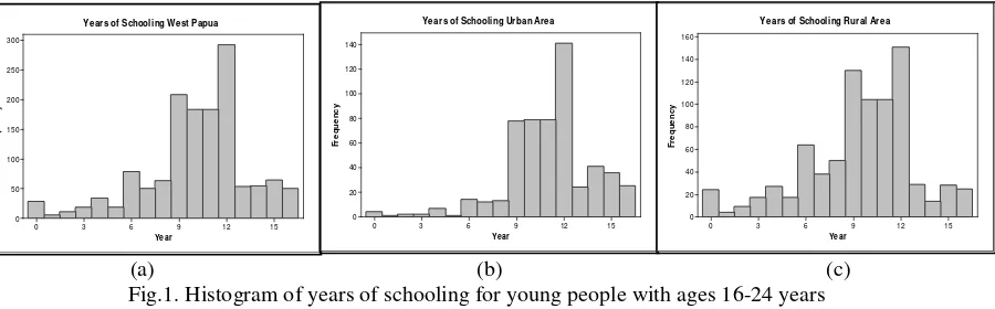
[image:6.595.82.532.294.434.2](a) (b) (c)
Fig.1. Histogram of years of schooling for young people with ages 16-24 years
Histogram on Fig. 1(a) reveals that the data patterns tend to be asymmetric. It indicates a multimodal nature of the data so that lead mixture distribution. In this study, components of mixture are considered by the status of county, namely urban and rural areas with the distribution pattern of data as shown in Fig. 1 (b) and (c).
Tab. 3. Goodness of Fit
Distribution West Papua Urban Rural Critical Value
Normal 25.536 9.4611 14.012 2,5018
Weibull 74.28 16.566 57.506 2,5018
Lognormal 120.47 29.102 83.742 2,5018
Log-Logistik 97.523 18.36 75.025 2,5018
Gamma 99.292 21.998 71.358 2,5018
Tab. 3 shows that the lowest value of Anderson-Darling statistic at 5% significance level is normal distribution for overall, urban and rural. This testing found that there was no corresponding distribution because the value of Anderson Darling statistic is greater than the critical value. However, much reliability modeling is based on the assumption that the data follow a weibull distribution which has non-negative number. Indication of mixture distribution can be considered by using weibull distribution approach for both areas. Weibull distribution has γ as shape parameter and λ as scale parameter.
In this case, the prior distribution used the conjugate prior, pseudo prior, and informative prior. Prior conjugate of weibull distribution is gamma distribution which comes from the exponential family. The normal distribution is used as a prior for β. Pseudo prior is used to determine initial parameter of
15 12 9 6 3 0 300 250 200 150 100 50 0 Year F r e q u e n c y
Years of Schooling West Papua
15 12 9 6 3 0 140 120 100 80 60 40 20 0 Year F r e q u e n c y
Years of Schooling Urban Area
15 12 9 6 3 0 160 140 120 100 80 60 40 20 0 Year F r e q u e n c y
conjugate prior which this initial is obtained from maximum likelihood method or frequentist way. Furthermore, all the information above results the informative prior for the next parameter estimation. The posterior which is used for parameter estimation of mixture weibull proportional hazards based on prior distribution and likelihood can be written as:
[image:7.595.93.497.129.384.2]p(γ,λ,β, e, π | t) ∝p(γ) p(λ) p(β) p(e) �∏�=1� ∑��=1������|��,��,��,����
Fig.2. Plot -ln [-ln S(t)] to the survival time
To assess whether the proportional hazards assumption is satisfied for either or both of these variables, we would need to compare log-log survival curves involving categories of these variables. The curves for each categorical variable are parallel and not intersect, as shown in Fig.2 we would conclude that the proportional hazards assumption is satisfied.
Tab.4. Parameter Estimation of Mixture Weibull Distribution
Parameter Mean Std.Dev 2.5% Median 97.5%
Phi[1] 0.4013 0.01308 0.3755 0.4012 0.4217
Phi[2] 0.5987 0.01308 0.5729 0.5988 0.6245
pGamma[1] 4.491 0.2271 4.164 4.498 4.839
pGamma[2] 2.726 0.08963 2.562 2.731 2.881
pLambda[1] 3.45x10⁻⁵ 4.64x10⁻⁴ 5.769x10⁻⁶ 1.394x10⁻⁵ 3.271x10⁻⁵
pLambda[2] 0.00176 7.44x10⁻⁴ 0.001163 0.001692 0.002568
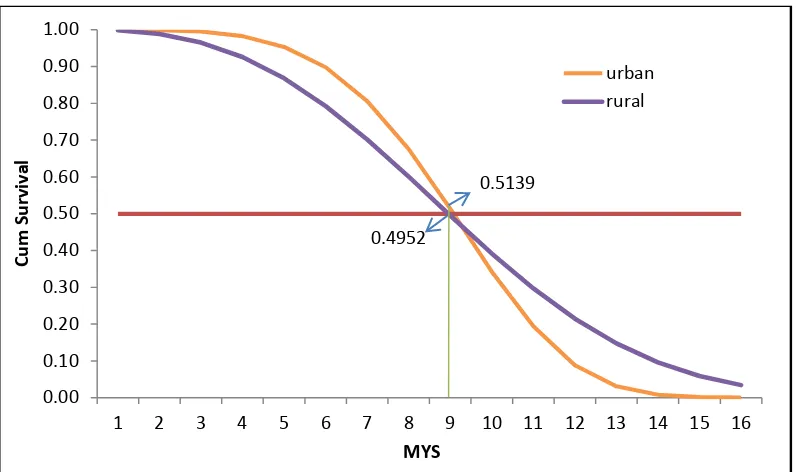
Fig.3. Plot of Survival Function in Urban and Rural Area
Calculation results of survival function with the parameter values obtained as shown in Fig.3. It appears that the value of survival function has decreased by increasing the years of schooling for both areas. The survival probability to have finished a study in junior high school level is 0.5027 or 50.70% for young people with age 16-24 years, where at each area are 0.5139 and 0.4952 for urban and rural area respectively. It means that urban area has a longer survival time to study than rural area.
Tab.5. Parameter Estimation of Mixture Weibull Proportional Hazards Model
Parameter Mean Std.Dev Exp (B) 2.5% Median 97.5%
b1[1] 0.1295 0.8978 1.1383 0.007077 0.1557 0.3099
b1[2] 0.02182 0.4322 1.0221 -0.1019 0.02412 0.1553
b2[1] -0.2856 0.6878 0.7516 -0.4218 -0.2536 -0.09363
b2[2] -0.0567 0.3515 0.9449 -0.1648 -0.04524 0.06082
b3[1] -0.3568 1.712 0.6999 -0.4128 -0.2556 -0.1014
b3[2] 0.05657 2.153 1.0582 0.03301 0.1643 0.29
b4_1[1] 0.2666 0.2905 1.3055 0.04319 0.2729 0.4764
b4_1[2] 0.4401 0.3891 1.5529 0.264 0.4422 0.6047
b4_2[1] 0.2232 0.2675 1.2501 0.02204 0.2364 0.4135
b4_2[2] 0.1998 0.252 1.2212 0.04374 0.2166 0.3652
b4_3[1] 0.1802 1.14 1.1975 0.003771 0.2157 0.4048
b4_3[2] 0.08618 0.2457 1.0900 -0.1054 0.08369 0.268
b5[1] -0.05267 0.5259 0.9487 -0.04892 0.001378 0.03777
b5[2] -0.02983 0.4149 0.9706 -0.02803 0.008322 0.03694
b6[1] -0.01435 0.1035 0.9858 -0.02398 -0.007555 0.006633
b6[2] -0.02047 0.1274 0.9797 -0.03262 -0.01122 0.006017
Based on the results as shown in Tab.5, not all parameters of the model are significant. The variables significantly influence the response if the credibility interval of median does not contain zero value. Therefore, the variables which significantly affect the years of schooling in urban area are gender
0.5139
0.4952
0.00 0.10 0.20 0.30 0.40 0.50 0.60 0.70 0.80 0.90 1.00
1 2 3 4 5 6 7 8 9 10 11 12 13 14 15 16
C
u
m S
u
rv
iv
a
l
MYS
urban
(X1), working activity (X2), marital status (X3), the education of householder at the lowest category
which they are not passed elementary school (X41), the education of householder at passed elementary
school category (X42) and the education of householder at passed junior high school category (X43).
Meanwhile, the variables which significantly affect the years of schooling in rural areas are marital status (X3), the education of householder at the lowest category which they are not passed elementary
school (X41), and the education of householder at passed elementary school category (X42). The results
also show that there is different effect of marital status in urban and rural area. The single status in rural area has longer time to study than married, but it does not occur in urban area. Beside, the contribution of urban and rural area are significantly affecting the years of schooling in West Papua province which have proportion about 0.4013 and 0.5987 respectively. Meanwhile, the number of household member and the average of household expenditure per capita have no significant effect to the years of schooling in West Papua Province.
Mathematically mixture proportional hazards model of each area can be written as:
1 1 2 3 41 42 43
5 4.491 1
( ) 0.4013 exp(0.1295 0.2856 0.3568 0.2666 0.2232 0.1802 )
x 3.45 x10 x 4.491
i i i i i i i
h t X X X X X X
t
− −
= − − + + +
2.726 1 2( ) 0.5987 exp(0.05657 3 0.4401 41 0.1998 42 ) x 0.00176 x 2.726
i i i i
h t = X + X + X t −
For recommendation, the government should give more attention to improve the education quality of young people especially in urban area. However, the rural area also needs to be improved because of the higher contribution to the years of schooling in West Papua.
4.
Conclusion
Rural areas were evidenced to contribute the years of schooling distribution higher than urban area up to 59.87 percent. The opportunity to obtain formal education to junior high school in urban area was greater than in rural area, but it went down faster in year 12-th or the senior high school level. In general, the factors affected the years of schooling in urban and rural area were diverse. In urban areas, the factors consisted of gender, working activity, marital status, and education level of the householder. Meanwhile, merely the marital status and education level of householder affected years of schooling in rural areas.
References
[1] G. Brunello and D. Checchib. School quality and family background in Italy. Economics of Education Review, 24:563–577, 2005.
[2] B. Santoso. Spline Multivariable and MARS Approach on Modeling Years of Schooling on The School Age Population in Papua province. Thesis, Institut Teknologi Sepuluh Nopember Surabaya, 2009.
[3] J. Qudsi. Mixture Survival Spasial Models for Years of Schooling on School Age 16-18 years in East Java 2012. Thesis, Institut Teknologi Sepuluh Nopember, Surabaya, 2015.
[4] G. McLachlan and K. E. Basford. Mixture Models Inference and Applications to Clustering. Marcel Dekker, 1988.
[5] N. Iriawan and S. P. Astuti. Mengolah Data Statistik dengan Mudah Menggunakan Minitab 14. Andi Offset, Yogyakarta. 2006.
[6] D. G. Kleinbaum and M. Klein. Survival Analysis: A Self Learning, 2nd Edition. Springer, 2005.
[7] E. Lee. Statistical Models and Methods for Lifetime Data. John Wiley and Sons Inc., 1992. [8] Zang. Survival Analysis. Wadsworth, 2008.
[10] J. M. Marin, K. L. Mengersen, and C.P. Robert. Bayesian Modelling and Inference on Mixtures of Distributions, Handbook of Statistics, volume 25, Elsevier, 2005.
[11] M. Stephen. Bayesian Metods for Mixture of Normal Distribution. Thesis, University of Oxford, UK, 1997.
[12] D. Gamerman. Markov Chain Monte Carlo. Chapman & Hall, 1997.
[13] N. Iriawan. Computationally Intensive Approaches to Inference in Neo-Normal Linier Models, Thesis Ph.D., CUT-Australia. 2000.
[14] G. E. P. Box and G. C. Tiao. Bayesian Inference in Statistical Analysis. Addison-Wesley, 1973. [15] I. Ntzoufras. Bayesian Modelling Using WinBUGS. John Willey and Sons Inc., 2009.
[16] B. P. Carlin and S. Chib. Bayesian model choice via Markov Chain Monte Carlo methods. Journal of The Royal Statistical Society, Vol. 57(3): page 473-484, 1995.
![Fig.2. Plot -ln [-ln S(t)] to the survival time](https://thumb-ap.123doks.com/thumbv2/123dok/893580.597203/7.595.93.497.129.384/fig-plot-ln-ln-s-t-survival-time.webp)